4. First steps and pymetamodels tutorials

First steps and tutorials on how to use pymetamodels can be found in this section,

• Tutorial case A01: “Sensitivity Analysis of a Coupled Function”

• Tutorial case A02: “Sensitivity Analysis of a Coupled Function, structure of data objects”

• Tutorial case A03: “Models and metamodels construction of a coupled function”

• Tutorial case A04: “Sensitivity analysis and metamodeling of Kursawe Functions”

• Tutorial case A05: “Sensitivity analysis and metamodeling of a damped oscillator”

• Tutorial case A06: “Minimization of the Kursawe Functions”

• Tutorial case A07: “Calibration of a damped oscillator”

• Tutorial case A08: “Building the configuration spreadsheet programatically”

• Tutorial case A09: “Loading DOEs from file, couple function case”

4.1. Tutorial case A01: “Sensitivity analysis of a coupled function”

Example of DOE design and sensitivity analysis for a coupled function.

The coupled function is defined as follows,

\begin{equation} Y = 0.5 \cdot X1+X2+0.5 \cdot X1 \cdot X2+5 \cdot sin(X3)+0.2 \cdot X4+0.1 \cdot X5 \end{equation}

The input and output variable for each of the analysis cases are define in the problem definition spreadsheet file (Download: Problem definition spreadsheet file). This definition spreadsheet includes the table with the main cases definition (Table 4.1.1), the table with model input variables (Table 4.1.2) and the table with output variables (Table 4.1.3).

Table 4.1.1 Main cases description for the coupled function tutorial

case	vars sheet	output sheet	samples	sensitivity method	comment
case_0	case_0_vars_sensi	case_out	50.0	DGSM
case_1	case_1_vars_sensi	case_out	50.0	RBD-Fast

Table 4.1.2 Main case input model variables description for the coupled function tutorial

variable	value	min	max	distribution	is_range	cov_un	ud	alias	comment	constrain	comment
X1	1.0	-3.14	3.14	unif	1	0.05	[-]	X1	None	0	var X1
X2	1.0	-3.14	3.14	unif	1	0.05	[-]	X2	None	0	var X2
X3	1.0	-3.14	3.14	unif	1	0.05	[-]	X3	None	0	var X3
X4	1.0	-3.14	3.14	unif	1	0.05	[-]	X4	None	0	var X4
X5	1.0	-3.14	3.14	unif	1	0.05	[-]	X5	None	0	var X5

Table 4.1.3 Main case output model variables description for the coupled function tutorial

variable	value	ud	comment	array
Y	None	m^3	function output	0

The analysis is performed with pymetamodels based on a basic analysis script as follows in test_analysis.py,

Listing 4.1.1 Coupled function test analysis. Sensitivity analysis

#!/usr/bin/env python3

## Analytical model,
##

import os, sys, random
import numpy as np
import gc

import pymetamodels
import coupled_function_model as model_obj

class analysis(object):

    """

    .. _model_coupled_function:

    **Synopsis:**
        * Analysis framework with pymetamodels

    """

    def __init__(self):

        ## Initial variables
        self.name = "coupled_function"
        self.folder_script = os.path.dirname(os.path.realpath(__file__))

        self.folder_path_inputs = self.folder_script

        self.folder_path_outputs = os.path.join(os.path.join(os.path.join(self.folder_script, os.pardir), "_examples_raw"),self.name + "_out")
        if not os.path.exists(self.folder_path_outputs): os.makedirs(self.folder_path_outputs)

        self.file_name_inputs = r"configuration_spreadsheet"
        self.file_name_outputs = r"outputs"

        ## Initialise 
        self.mita = pymetamodels.load()
        self.mita.logging_start(self.folder_path_outputs)        

    def run_model(self):

        ## Inputs load
        folder_path = self.folder_path_inputs
        file_name = self.file_name_inputs
        self.mita.read_xls_case(folder_path, file_name, sheet="cases", col_start = 0, row_start = 1, tit_row = 0 )

        ## Sampling
        for case in self.mita.keys():

            ## Run samplimg cases
            self.mita.run_sampling_routine(case)

            ## Run / Load model
            self.model_iteration(case, model_obj)

            ## Sensitivity analysis
            self.mita.run_sensitivity_analisis(case)
            #self.mita.print_dict(self.mita.SiY(case))

        ##
        self.mita.run_sensitivity_normalization()

        ## Ploting and others
        for case in self.mita.keys():

            ## Plot cross varible relation in the sensitivity analysis
            self.mita.output_plts_sensitivity(self.folder_path_outputs, case)

        ## Output variables save
        folder_path = self.folder_path_outputs
        file_name = self.file_name_outputs
        out_path = self.mita.output_xls(folder_path, file_name, col_start = 0, tit_row = 0)

    def model_iteration(self, case, _model_obj):

        ## Model iteration to generate Y doe output values
        doeX = self.mita.doeX(case)
        doeY = self.mita.doeY(case)
        vars_in = self.mita.vars_parameter_matrix(case)
        case_dict = self.mita.case[case]
        samples = len(doeX[list(doeX.keys())[0]])

        for ii in range(0, samples):

            obj_model = _model_obj.model_obj()

            # initialize dictionaries
            obj_model.doeX = doeX
            obj_model.doeY = doeY
            obj_model.case_dict = case_dict
            obj_model.ii = ii
            obj_model.vars_in = vars_in

            # add variables as atributes
            for key in obj_model.doeX.keys():
                setattr(obj_model, key, obj_model.doeX[key][obj_model.ii])

            # run the model for ii sample
            obj_model.run_model()

if __name__ == "__main__":

    analysis = analysis()

    analysis.run_model()

The analysis frameworks iterates the model defined in a secondary file as follows in coupled_function_model.py,

Listing 4.1.2 Coupled function model code block. Sensitivity analysis

#!/usr/bin/env python3

## coupled function
##

import os, sys, random
import numpy as np
from math import *

class model_obj(object):

    """

    .. _model_id_001_coupled_function:

    **Coupled_function**

    :platform: Unix, Windows
    :synopsis: coupled fuction
    :author: FLC

    :Dependences:

    """

    def __init__(self):

        ## Initial variables
        self.doeX = None
        self.doeY = None
        self.case_dict = None
        self.ii = None

    def run_model(self):

        # variables
        X1 = self.doeX["X1"][self.ii]
        X2 = self.doeX["X2"][self.ii]
        X3 = self.doeX["X3"][self.ii]
        X4 = self.doeX["X4"][self.ii]
        X5 = self.doeX["X5"][self.ii]

        # calculations
        Y =  0.5*X1+X2+0.5*X1*X2+5*sin(X3)+0.2*X4+0.1*X5

        # outputs
        self.doeY["Y"][self.ii] = Y

        pass

Running the analysis script generates and output results files containing the DOEX input data, the DOEY output data and the senstitivity analysis,

Download: Output spreadsheet file

The console output of running the tutorial script is as follow,

Msg: Case case_0 sampling value 64 by DGSM. DOEX shape (384, 5)

Msg: Case case_1 sampling value 64 by latin Hypercube for RBD-FAST. DOEX shape (64, 5)

Plot create ID: cross_X1_X2_case_0

Plot create ID: cross_X1_X3_case_0

Plot create ID: cross_X1_X4_case_0

Plot create ID: cross_X1_X5_case_0

Plot create ID: cross_X2_X3_case_0

Plot create ID: cross_X2_X4_case_0

Plot create ID: cross_X2_X5_case_0

Plot create ID: cross_X3_X4_case_0

Plot create ID: cross_X3_X5_case_0

Plot create ID: cross_X4_X5_case_0

Msg: Cross DOEX variable sampling combinations and sensitivity analisys plotted

Plot create ID other: sensi_case_0_Y

Msg: Sensitivity histograms plotted

Plot create ID: cross_X1_X2_case_1

Plot create ID: cross_X1_X3_case_1

Plot create ID: cross_X1_X4_case_1

Plot create ID: cross_X1_X5_case_1

Plot create ID: cross_X2_X3_case_1

Plot create ID: cross_X2_X4_case_1

Plot create ID: cross_X2_X5_case_1

Plot create ID: cross_X3_X4_case_1

Plot create ID: cross_X3_X5_case_1

Plot create ID: cross_X4_X5_case_1

Msg: Cross DOEX variable sampling combinations and sensitivity analisys plotted

Plot create ID other: sensi_case_1_Y

Msg: Sensitivity histograms plotted

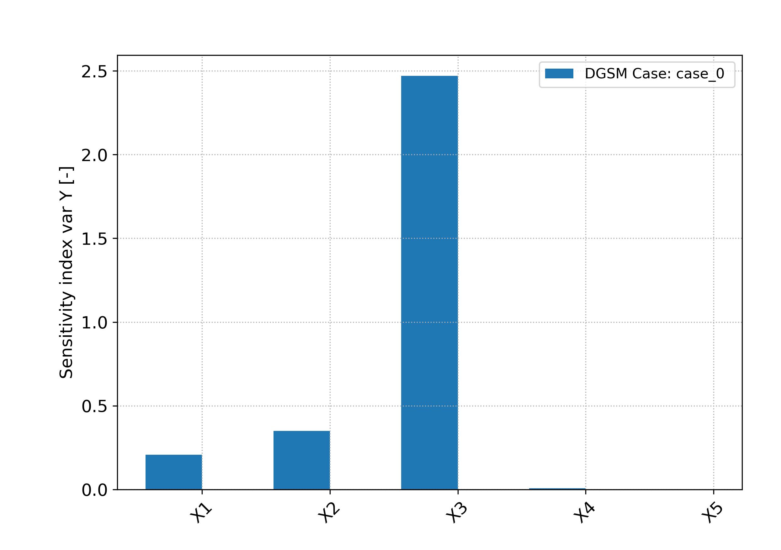
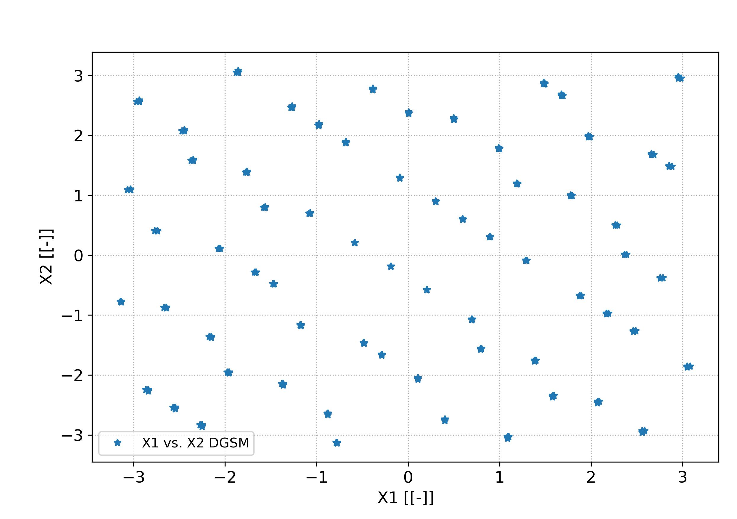
The function output_plts_sensitivity() generates several plots showing the DOEX variables correlation and a summary of the sensitivity analysis. For example this can be seen in Fig. 4.1.1 and Fig. 4.1.2. This plot are located in the output folder.

Fig. 4.1.1 Sensitivity bar plot for case_0. Tutorial A01

Fig. 4.1.2 Cross represenation of variable X1 versus X2 in case_0. Tutorial A01

4.2. Tutorial case A02: “Sensitivity analysis of a coupled function, structure of data objects”

Based on the DOE design and sensitivity analysis for a coupled function described in the previous Tutorial case. In this tutorial are described the data object structure. For this purpose the different data object structure is access and printed.

The input and output variable for each of the analysis cases are define in the problem definition spreadsheet file (Download: Problem definition spreadsheet file). This definition spreadsheet includes the table with the main cases definition (Table 4.1.1), the table with model input variables (Table 4.1.2) and the table with output variables (Table 4.1.3).

Table 4.2.1 Main cases description for the coupled function tutorial data structure

case	vars sheet	output sheet	samples	sensitivity method	comment
case_1	case_1_vars_sensi	case_out	50.0	RBD-Fast

Table 4.2.2 Main case input model variables description for the coupled function tutorial data structure

variable	value	min	max	distribution	is_range	cov_un	ud	alias	comment	constrain	comment
X1	1.0	-3.14	3.14	unif	1	0.05	[-]	X1	None	0	var X1
X2	1.0	-3.14	3.14	unif	1	0.05	[-]	X2	None	0	var X2
X3	1.0	-3.14	3.14	unif	1	0.05	[-]	X3	None	0	var X3
X4	1.0	-3.14	3.14	unif	1	0.05	[-]	X4	None	0	var X4
X5	1.0	-3.14	3.14	unif	1	0.05	[-]	X5	None	0	var X5

Table 4.2.3 Main case output model variables description for the coupled function tutorial data structure

variable	value	ud	comment	array
Y	None	m^3	function output	0

The code to print the data structure objects are described in the script as follows in test_analysis.py,

Listing 4.2.1 Coupled function test analysis. Structure of data objects

#!/usr/bin/env python3

## Analytical model,
##

import os, sys, random
import numpy as np
import gc

import pymetamodels
import coupled_function_model as model_obj

class analysis(object):

    """

    .. _model_coupled_function_data_struct:

    **Synopsis:**
        * Analysis framework with pymetamodels

    """

    def __init__(self):

        ## Initial variables
        self.name = "coupled_function_data_struct"
        self.folder_script = os.path.dirname(os.path.realpath(__file__))

        self.folder_path_inputs = self.folder_script

        self.folder_path_outputs = os.path.join(os.path.join(os.path.join(self.folder_script, os.pardir), "_examples_raw"),self.name + "_out")
        if not os.path.exists(self.folder_path_outputs): os.makedirs(self.folder_path_outputs)

        self.file_name_inputs = r"configuration_spreadsheet"
        self.file_name_outputs = r"outputs"

        ## Initialise 
        self.mita = pymetamodels.load()
        self.mita.logging_start(self.folder_path_outputs)        

    def run_model(self):

        ## Inputs load
        folder_path = self.folder_path_inputs
        file_name = self.file_name_inputs
        self.mita.read_xls_case(folder_path, file_name, sheet="cases", col_start = 0, row_start = 1, tit_row = 0 )

        ## Sampling
        for case in self.mita.keys():

            ## Run samplimg cases
            self.mita.run_sampling_routine(case)

            ## Run / Load model
            self.model_iteration(case, model_obj)

            ## Sensitivity analysis
            self.mita.run_sensitivity_analisis(case)

        ##
        self.mita.run_sensitivity_normalization()

        ## Print data structure for investigation
        for case in self.mita.keys():
            print("*:-)* Printing data object structure for case %s" % case)
            self.mita.print_structure(case)

        ## Print data structure for investigation
        for case in self.mita.keys():
            print("*:-)* Printing DOEX data object structure for case %s" % case)
            self.mita.print_dict(self.mita.doeX(case))

        ## Print data structure for investigation
        for case in self.mita.keys():
            print("*:-)* Printing DOEY data object structure for case %s" % case)
            self.mita.print_dict(self.mita.doeX(case))

        ## Print data structure for investigation
        for case in self.mita.keys():
            print("*:-)* Printing sensitivity SiY data object structure for case %s" % case)
            self.mita.print_dict(self.mita.SiY(case))

        ## Print data structure for investigation
        for case in self.mita.keys():
            print("*:-)* Printing parameters values for each input variable data object structure for case %s" % case)
            self.mita.print_dict(self.mita.vars_parameter_matrix(case))



        ## Output variables save
        folder_path = self.folder_path_outputs
        file_name = self.file_name_outputs
        out_path = self.mita.output_xls(folder_path, file_name, col_start = 0, tit_row = 0)

    def model_iteration(self, case, _model_obj):

        ## Model iteration to generate Y doe output values
        doeX = self.mita.doeX(case)
        doeY = self.mita.doeY(case)
        vars_in = self.mita.vars_parameter_matrix(case)
        case_dict = self.mita.case[case]
        samples = len(doeX[list(doeX.keys())[0]])

        for ii in range(0, samples):

            obj_model = _model_obj.model_obj()

            # initialize dictionaries
            obj_model.doeX = doeX
            obj_model.doeY = doeY
            obj_model.case_dict = case_dict
            obj_model.ii = ii
            obj_model.vars_in = vars_in

            # add variables as atributes
            for key in obj_model.doeX.keys():
                setattr(obj_model, key, obj_model.doeX[key][obj_model.ii])

            # run the model for ii sample
            obj_model.run_model()

if __name__ == "__main__":

    analysis = analysis()

    analysis.run_model()

The console output of running the tutorial script is as follow,

Msg: Case case_1 sampling value 32 by latin Hypercube for RBD-FAST. DOEX shape (32, 5)

*:-)* Printing data object structure for case case_1

Msg: Data dict structure

Msg:   case = case_1

Msg:   vars sheet = case_1_vars_sensi

Msg:   output sheet = case_out

Msg:   samples = 32.0

Msg:   sensitivity method = RBD-Fast

Msg:   comment =

Msg:   [vars]

Msg:     X1 = 1.0

Msg:     [[op_X1]]

Msg:       value = 1.0

Msg:       min = -3.14

Msg:       max = 3.14

Msg:       distribution = unif

Msg:       is_range = 1

Msg:       cov_un = 0.05

Msg:       ud = [-]

Msg:       alias = X1

Msg:       comment = var X1

Msg:       constrain = 0

Msg:     X2 = 1.0

Msg:     [[op_X2]]

Msg:       value = 1.0

Msg:       min = -3.14

Msg:       max = 3.14

Msg:       distribution = unif

Msg:       is_range = 1

Msg:       cov_un = 0.05

Msg:       ud = [-]

Msg:       alias = X2

Msg:       comment = var X2

Msg:       constrain = 0

Msg:     X3 = 1.0

Msg:     [[op_X3]]

Msg:       value = 1.0

Msg:       min = -3.14

Msg:       max = 3.14

Msg:       distribution = unif

Msg:       is_range = 1

Msg:       cov_un = 0.05

Msg:       ud = [-]

Msg:       alias = X3

Msg:       comment = var X3

Msg:       constrain = 0

Msg:     X4 = 1.0

Msg:     [[op_X4]]

Msg:       value = 1.0

Msg:       min = -3.14

Msg:       max = 3.14

Msg:       distribution = unif

Msg:       is_range = 1

Msg:       cov_un = 0.05

Msg:       ud = [-]

Msg:       alias = X4

Msg:       comment = var X4

Msg:       constrain = 0

Msg:     X5 = 1.0

Msg:     [[op_X5]]

Msg:       value = 1.0

Msg:       min = -3.14

Msg:       max = 3.14

Msg:       distribution = unif

Msg:       is_range = 1

Msg:       cov_un = 0.05

Msg:       ud = [-]

Msg:       alias = X5

Msg:       comment = var X5

Msg:       constrain = 0

Msg:   [vars_out]

Msg:     Y = None

Msg:     [[op_Y]]

Msg:       value = None

Msg:       ud = m^3

Msg:       comment = function output

Msg:       array = 0

Msg:   [problem]

Msg:     num_vars = 5

Msg:     names = ['X1', 'X2', 'X3', 'X4', 'X5']

Msg:     bounds = [[-3.14, 3.14], [-3.14, 3.14], [-3.14, 3.14], [-3.14, 3.14], [-3.14, 3.14]]

Msg:     dists = ['unif', 'unif', 'unif', 'unif', 'unif']

Msg:   [DOE_X]

Msg:     X1 = [-1.59159879 -2.37095574 -2.71348644  1.22365411  2.82674911  0.2999615

  1.64725384  3.06161963  0.0742446  -2.28582998 -0.5587558  -1.82735767

 -1.31195326 -0.73077891  0.75394008 -0.99513504  0.8585848   2.45169679

  1.04023371  2.00955945 -3.0356118   1.89134424  1.49386002 -1.48587271

 -0.3298623   2.27657763 -2.14167914  0.47383463  2.55339845 -2.79819403

 -0.13323825 -0.80025798]

Msg:     X2 = [-1.49551768 -0.8232943   1.45585999 -2.96500852 -2.79608774  1.68019528

  1.81664636  2.22034641 -1.98682384 -1.00425972  2.66093103  2.76958816

 -2.20322023  0.13209743  0.7739977  -2.46343011 -1.25010436 -1.81424892

  2.40325057  0.87549163  0.35403306 -0.29919076  0.50626936 -0.70882351

 -0.02008361  3.11491833 -1.63528101 -0.55444911  1.10362982  2.04131733

  1.29687707 -2.63321811]

Msg:     X3 = [ 3.09699711  0.36966734 -0.57002289  1.50708007 -2.06922857  2.59258339

  0.19526522  1.64727312  1.96053652  0.97968859  2.81016127  2.53623619

 -3.00942706 -0.03068597 -0.92978557  2.224929    0.72726221  1.15537941

  1.23089618 -2.69491643 -2.7600673   2.02552516 -1.70788011 -2.27872345

 -2.36979067 -1.83677336 -0.73435615 -1.33261221 -1.01794021  0.53264105

 -1.41922755 -0.27131973]

Msg:     X4 = [-1.11656159  2.38923358 -2.75328799 -0.73142989  1.9493782  -0.82977894

  2.66457292  1.62690883  1.13595146 -0.56011449 -3.02408628  1.28223654

 -1.5666057   0.72028    -1.76033609 -0.12151199 -2.11662127 -2.18896799

 -0.21834053 -2.73883853  0.8447891   1.56912015 -1.87223673  2.04052934

  0.05035915 -2.51172914  3.03296838  2.30608184 -1.31902097  2.8707176

  0.57524509  0.28542285]

Msg:     X5 = [ 1.77889941 -1.99855931 -2.70658724 -2.47096652  3.0536835  -1.52908215

 -1.23152489  2.79263289  1.12450616 -2.90457174 -2.27649904 -0.88224136

  0.80567234 -1.69888088 -0.37545943 -0.77885064 -3.05102585  2.26839659

  0.55485414  1.74350232  1.37418039  0.02608228  0.3231309  -0.18227989

  0.60608273  1.31272188  1.98604421  2.60130571 -1.80306878 -0.54575217

  2.53868527 -1.10464129]

Msg:   [DOE_Y]

Msg:     Y = [-0.9237036   1.05174211 -5.39568432  0.42921752 -9.031054    4.37252071

  5.5164078  12.74011474  2.94122292  2.74974805  2.43266487  2.33889456

 -2.30559556 -0.46079688 -2.95433012  2.13041757  1.23823595  1.55139212

  8.89909567  0.22667888 -3.25643334  5.17187807 -3.66388073 -4.33382832

 -3.59816108  2.60362946 -3.50034583 -4.58638352 -0.90991966  0.84483907

 -3.42989846 -3.37311535]

Msg:   [Si_Y]

Msg:     [[Y]]

Msg:       S1 = [-0.8285000582672463, 0.1440109719362379, 0.6543986801275722, -0.08063536354778456, -0.08401437790256483]

Msg:       S1_conf = [0.0, 0.0, 0.0, 0.0, 0.0]

Msg:       names = ['X1', 'X2', 'X3', 'X4', 'X5']

*:-)* Printing DOEX data object structure for case case_1

Msg:   X1 = [-1.59159879 -2.37095574 -2.71348644  1.22365411  2.82674911  0.2999615

  1.64725384  3.06161963  0.0742446  -2.28582998 -0.5587558  -1.82735767

 -1.31195326 -0.73077891  0.75394008 -0.99513504  0.8585848   2.45169679

  1.04023371  2.00955945 -3.0356118   1.89134424  1.49386002 -1.48587271

 -0.3298623   2.27657763 -2.14167914  0.47383463  2.55339845 -2.79819403

 -0.13323825 -0.80025798]

Msg:   X2 = [-1.49551768 -0.8232943   1.45585999 -2.96500852 -2.79608774  1.68019528

  1.81664636  2.22034641 -1.98682384 -1.00425972  2.66093103  2.76958816

 -2.20322023  0.13209743  0.7739977  -2.46343011 -1.25010436 -1.81424892

  2.40325057  0.87549163  0.35403306 -0.29919076  0.50626936 -0.70882351

 -0.02008361  3.11491833 -1.63528101 -0.55444911  1.10362982  2.04131733

  1.29687707 -2.63321811]

Msg:   X3 = [ 3.09699711  0.36966734 -0.57002289  1.50708007 -2.06922857  2.59258339

  0.19526522  1.64727312  1.96053652  0.97968859  2.81016127  2.53623619

 -3.00942706 -0.03068597 -0.92978557  2.224929    0.72726221  1.15537941

  1.23089618 -2.69491643 -2.7600673   2.02552516 -1.70788011 -2.27872345

 -2.36979067 -1.83677336 -0.73435615 -1.33261221 -1.01794021  0.53264105

 -1.41922755 -0.27131973]

Msg:   X4 = [-1.11656159  2.38923358 -2.75328799 -0.73142989  1.9493782  -0.82977894

  2.66457292  1.62690883  1.13595146 -0.56011449 -3.02408628  1.28223654

 -1.5666057   0.72028    -1.76033609 -0.12151199 -2.11662127 -2.18896799

 -0.21834053 -2.73883853  0.8447891   1.56912015 -1.87223673  2.04052934

  0.05035915 -2.51172914  3.03296838  2.30608184 -1.31902097  2.8707176

  0.57524509  0.28542285]

Msg:   X5 = [ 1.77889941 -1.99855931 -2.70658724 -2.47096652  3.0536835  -1.52908215

 -1.23152489  2.79263289  1.12450616 -2.90457174 -2.27649904 -0.88224136

  0.80567234 -1.69888088 -0.37545943 -0.77885064 -3.05102585  2.26839659

  0.55485414  1.74350232  1.37418039  0.02608228  0.3231309  -0.18227989

  0.60608273  1.31272188  1.98604421  2.60130571 -1.80306878 -0.54575217

  2.53868527 -1.10464129]

*:-)* Printing DOEY data object structure for case case_1

Msg:   X1 = [-1.59159879 -2.37095574 -2.71348644  1.22365411  2.82674911  0.2999615

  1.64725384  3.06161963  0.0742446  -2.28582998 -0.5587558  -1.82735767

 -1.31195326 -0.73077891  0.75394008 -0.99513504  0.8585848   2.45169679

  1.04023371  2.00955945 -3.0356118   1.89134424  1.49386002 -1.48587271

 -0.3298623   2.27657763 -2.14167914  0.47383463  2.55339845 -2.79819403

 -0.13323825 -0.80025798]

Msg:   X2 = [-1.49551768 -0.8232943   1.45585999 -2.96500852 -2.79608774  1.68019528

  1.81664636  2.22034641 -1.98682384 -1.00425972  2.66093103  2.76958816

 -2.20322023  0.13209743  0.7739977  -2.46343011 -1.25010436 -1.81424892

  2.40325057  0.87549163  0.35403306 -0.29919076  0.50626936 -0.70882351

 -0.02008361  3.11491833 -1.63528101 -0.55444911  1.10362982  2.04131733

  1.29687707 -2.63321811]

Msg:   X3 = [ 3.09699711  0.36966734 -0.57002289  1.50708007 -2.06922857  2.59258339

  0.19526522  1.64727312  1.96053652  0.97968859  2.81016127  2.53623619

 -3.00942706 -0.03068597 -0.92978557  2.224929    0.72726221  1.15537941

  1.23089618 -2.69491643 -2.7600673   2.02552516 -1.70788011 -2.27872345

 -2.36979067 -1.83677336 -0.73435615 -1.33261221 -1.01794021  0.53264105

 -1.41922755 -0.27131973]

Msg:   X4 = [-1.11656159  2.38923358 -2.75328799 -0.73142989  1.9493782  -0.82977894

  2.66457292  1.62690883  1.13595146 -0.56011449 -3.02408628  1.28223654

 -1.5666057   0.72028    -1.76033609 -0.12151199 -2.11662127 -2.18896799

 -0.21834053 -2.73883853  0.8447891   1.56912015 -1.87223673  2.04052934

  0.05035915 -2.51172914  3.03296838  2.30608184 -1.31902097  2.8707176

  0.57524509  0.28542285]

Msg:   X5 = [ 1.77889941 -1.99855931 -2.70658724 -2.47096652  3.0536835  -1.52908215

 -1.23152489  2.79263289  1.12450616 -2.90457174 -2.27649904 -0.88224136

  0.80567234 -1.69888088 -0.37545943 -0.77885064 -3.05102585  2.26839659

  0.55485414  1.74350232  1.37418039  0.02608228  0.3231309  -0.18227989

  0.60608273  1.31272188  1.98604421  2.60130571 -1.80306878 -0.54575217

  2.53868527 -1.10464129]

*:-)* Printing sensitivity SiY data object structure for case case_1

Msg:   [Y]

Msg:     S1 = [-0.8285000582672463, 0.1440109719362379, 0.6543986801275722, -0.08063536354778456, -0.08401437790256483]

Msg:     S1_conf = [0.0, 0.0, 0.0, 0.0, 0.0]

Msg:     names = ['X1', 'X2', 'X3', 'X4', 'X5']

*:-)* Printing parameters values for each input variable data object structure for case case_1

Msg:   [X1]

Msg:     value = 1.0

Msg:     min = -3.14

Msg:     max = 3.14

Msg:     distribution = unif

Msg:     is_range = 1

Msg:     cov_un = 0.05

Msg:     ud = [-]

Msg:     alias = X1

Msg:   [X2]

Msg:     value = 1.0

Msg:     min = -3.14

Msg:     max = 3.14

Msg:     distribution = unif

Msg:     is_range = 1

Msg:     cov_un = 0.05

Msg:     ud = [-]

Msg:     alias = X2

Msg:   [X3]

Msg:     value = 1.0

Msg:     min = -3.14

Msg:     max = 3.14

Msg:     distribution = unif

Msg:     is_range = 1

Msg:     cov_un = 0.05

Msg:     ud = [-]

Msg:     alias = X3

Msg:   [X4]

Msg:     value = 1.0

Msg:     min = -3.14

Msg:     max = 3.14

Msg:     distribution = unif

Msg:     is_range = 1

Msg:     cov_un = 0.05

Msg:     ud = [-]

Msg:     alias = X4

Msg:   [X5]

Msg:     value = 1.0

Msg:     min = -3.14

Msg:     max = 3.14

Msg:     distribution = unif

Msg:     is_range = 1

Msg:     cov_un = 0.05

Msg:     ud = [-]

Msg:     alias = X5

4.3. Tutorial case A03: “Models and metamodels construction of a coupled function”

In this tutorial are described the construction of the model and metamodels, as well as the default plotting of them. For this purpose is used the DOE design and sensitivity analysis for a coupled function described in the previous tutorial case.

The code to print the data structure objects are described in the script as follows in test_analysis.py,

Listing 4.3.1 Coupled function test analysis. Metamodels

#!/usr/bin/env python3

## Analytical model,
##

import os, sys, random
import numpy as np
import gc

import pymetamodels
import coupled_function_model as model_obj

class analysis(object):

    """

    .. _model_coupled_function_metamodel:

    **Synopsis:**
        * Analysis framework with pymetamodels
        * Coupled function tutorial

    """

    def __init__(self):

        ## Initial variables
        self.name = "coupled_function_metamodel"
        self.folder_script = os.path.dirname(os.path.realpath(__file__))

        self.folder_path_inputs = self.folder_script

        self.folder_path_outputs = os.path.join(os.path.join(os.path.join(self.folder_script, os.pardir), "_examples_raw"),self.name + "_out")
        if not os.path.exists(self.folder_path_outputs): os.makedirs(self.folder_path_outputs)

        self.file_name_inputs = r"configuration_spreadsheet"
        self.file_name_outputs = r"outputs"

        ## Initialise 
        self.mita = pymetamodels.load()
        self.mita.logging_start(self.folder_path_outputs)        

    def run_model(self):

        ## Inputs load
        folder_path = self.folder_path_inputs
        file_name = self.file_name_inputs
        self.mita.read_xls_case(folder_path, file_name, sheet="cases", col_start = 0, row_start = 1, tit_row = 0 )

        ## Sampling
        for case in self.mita.keys():

            ## Run samplimg cases
            self.mita.run_sampling_routine(case)

            ## Run / Load model
            self.model_iteration(case, model_obj)

            ## Sensitivity analysis
            self.mita.run_sensitivity_analisis(case)

            ## Metamodeling construction
            #self.mita.run_metamodel_construction(case, scheme = "general")
            self.mita.run_metamodel_construction(case, scheme = "general_fast")

        ##
        self.mita.run_sensitivity_normalization()

        ## Ploting and others
        for case in self.mita.keys():

            ## Plots cross varible relation in the sensitivity analysis
            self.mita.output_plts_sensitivity(self.folder_path_outputs, case)

            ## Plots showing the model DOEX and DOEY variables relationship 2D XY
            self.mita.output_plts_models_XY(self.folder_path_outputs, case)

            ## Residual values plots
            self.mita.output_plts_models_residuals_plot(self.folder_path_outputs, case)

            ## Plots showing the model DOEX and DOEY variables relationship 3D XYZ
            self.mita.output_plts_models_XYZ(self.folder_path_outputs, case, scatter=False)

        ## Output variables save
        folder_path = self.folder_path_outputs
        file_name = self.file_name_outputs
        out_path = self.mita.output_xls(folder_path, file_name, col_start = 0, tit_row = 0)

    def model_iteration(self, case, _model_obj):

        ## Model iteration to generate Y doe output values
        doeX = self.mita.doeX(case)
        doeY = self.mita.doeY(case)
        vars_in = self.mita.vars_parameter_matrix(case)
        case_dict = self.mita.case[case]
        samples = len(doeX[list(doeX.keys())[0]])

        for ii in range(0, samples):

            obj_model = _model_obj.model_obj()

            # initialize dictionaries
            obj_model.doeX = doeX
            obj_model.doeY = doeY
            obj_model.case_dict = case_dict
            obj_model.ii = ii
            obj_model.vars_in = vars_in

            # add variables as atributes
            for key in obj_model.doeX.keys():
                setattr(obj_model, key, obj_model.doeX[key][obj_model.ii])

            # run the model for ii sample
            obj_model.run_model()

if __name__ == "__main__":

    analysis = analysis()

    analysis.run_model()

The function run_metamodel_construction() is included in the code to execute the routines related with the metamodeling construction of the DOEY as function of the DOEX data. This functions allows to choose different metamodeling schemas. This schemas perform a robust metamodeling search and find to determine the most adequate metamodeling ML model. Once the ML metamodel is determined allows to predict any data in the ranges of the DOEX and DOEY training values.

The function output_plts_models_residuals_plot() plots the residual values of the ML metamodel DOEY predictions in comparison with the ground truth DOEY values showing the regression score between the data and the predictions. An example can be seen in Fig. 4.3.3.

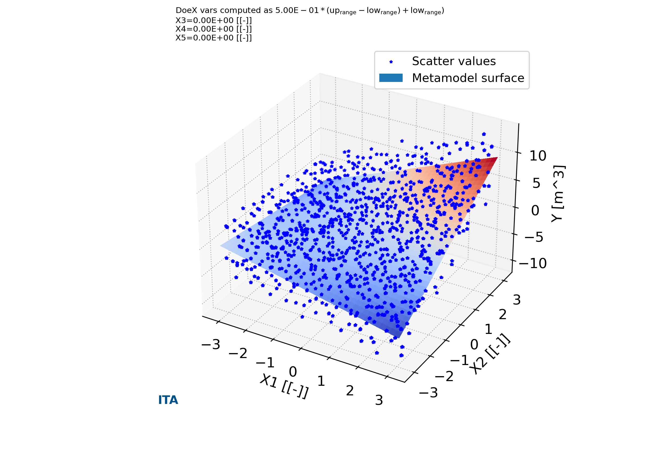
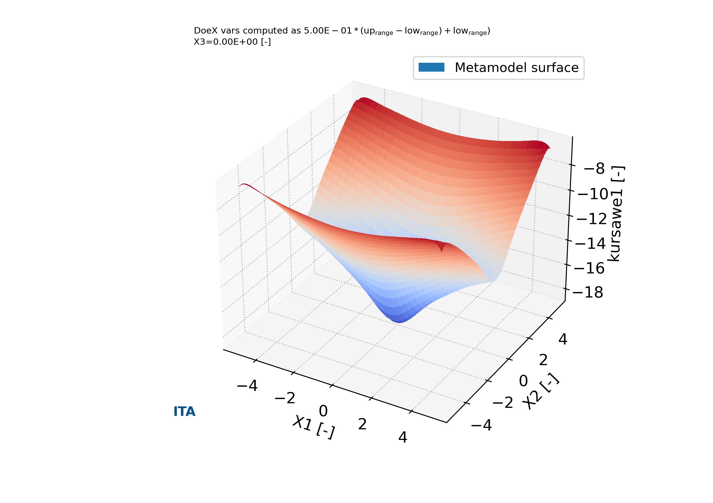
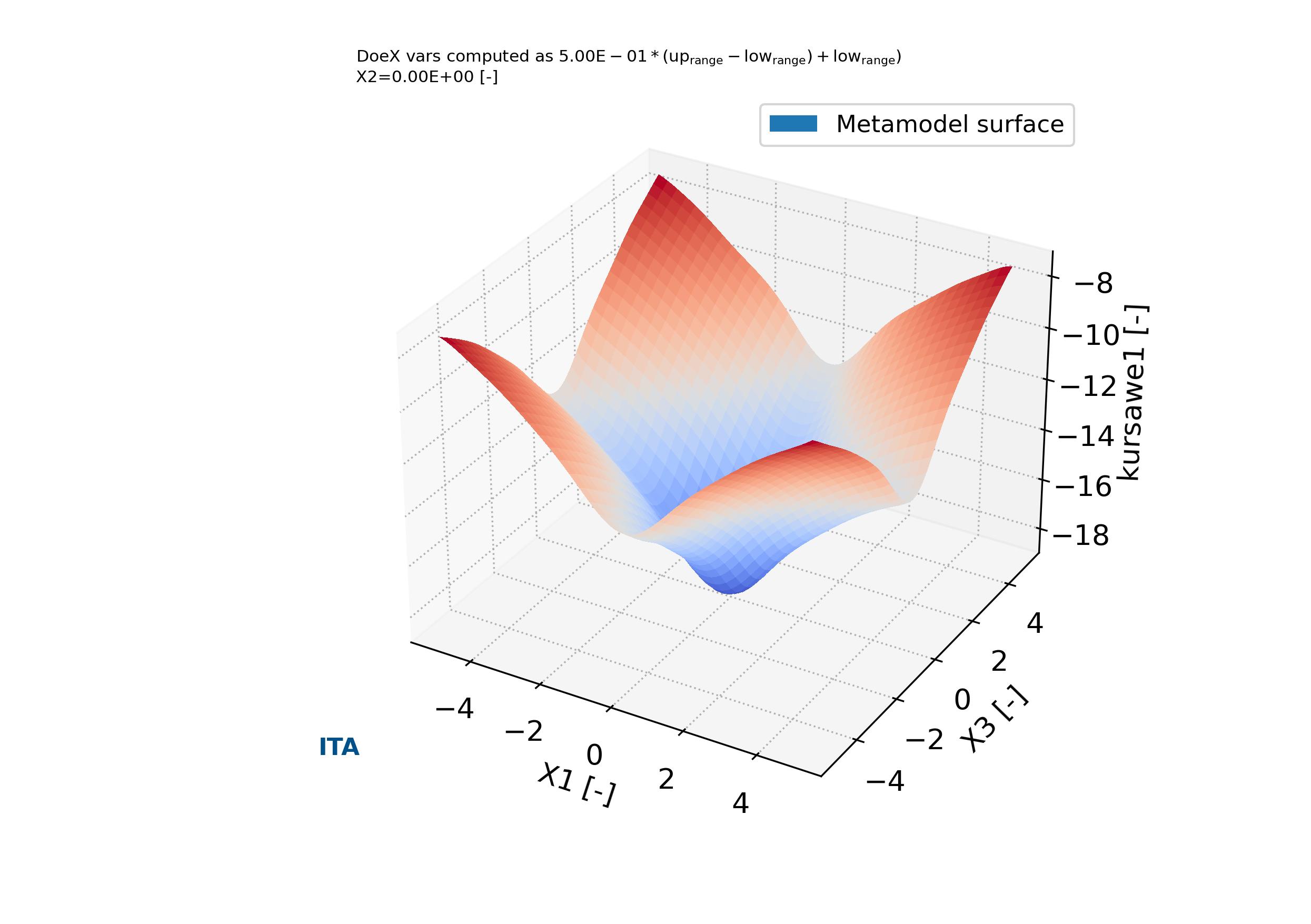
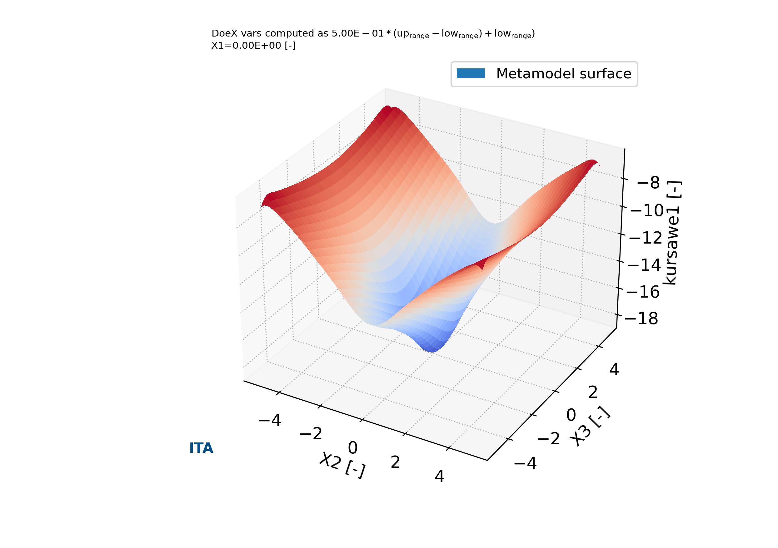
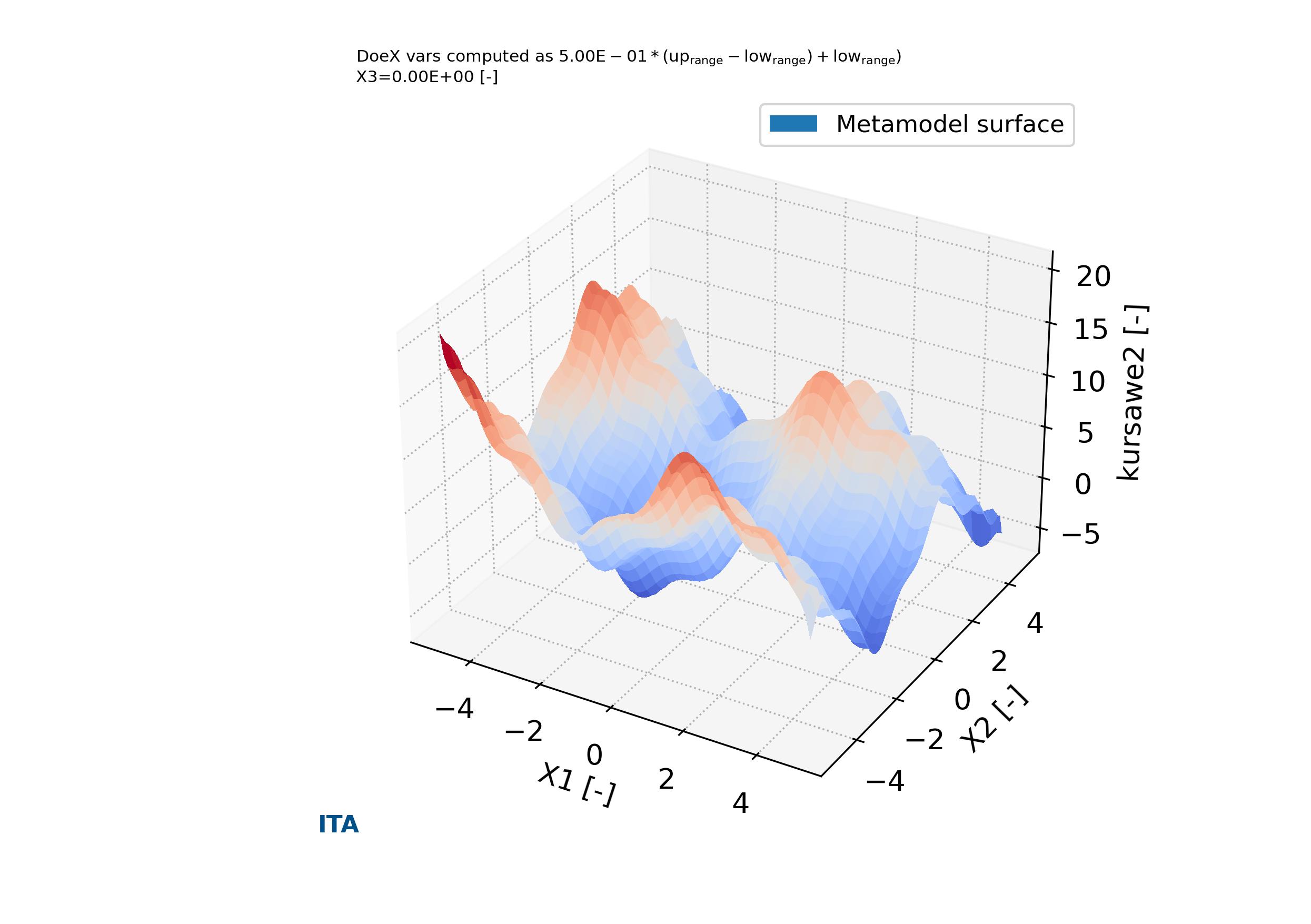
In addition, the function output_plts_models_XYZ() plot all the combinations of XYZ plots showing the prediction surfaces constructed using the ML metamodel. An example can be seen in Fig. 4.3.1 and Fig. 4.3.2.

Fig. 4.3.1 Metamodels surface of variable X1 versus X2 versus Y in case_1. Tutorial A03

Fig. 4.3.2 Metamodels surface of variable X2 versus X3 versus Y in case_1. Tutorial A03

Fig. 4.3.3 Metamodels residual plot Y values versus predictions in case_1. Tutorial A03

4.4. Tutorial case A04: “Sensitivity analysis and metamodeling of Kursawe Functions”

In this tutorial are described the construction of the model, sensitivity analysis and metamodels, as well as the default plotting of them. For this purpose is used the DOE design and sensitivity analysis for a coupled function described in the previous tutorial case as a base line. The Kursawe Functions are define by three variables \(X_1, X_2, X_3\) and two output functions \(f_{kursawe1}, f_{kursawe2}\),

\begin{equation} \begin{cases} f_{kursawe1}(x) = \sum_{i=1}^{2} -10 \cdot e^{-0.2 \cdot \sqrt{X_{i}^{2} + X_{i+1}^{2} }} \\ f_{kursawe2}(x) = \sum_{i=1}^{3} \left|X_i\right|^{0.8} + 5 \cdot sin (X_{i}^3) \\ where;\\ -5 <= X_i <= 5, i=1,...,n \end{cases} \end{equation}

The input and output variable for each of the analysis cases are define in the problem definition spreadsheet file (Download: Problem definition spreadsheet file).

The analysis is performed with pymetamodels based on a basic analysis script as follows in test_analysis.py,

Listing 4.4.1 Kursawe Functions test analysis. Sensitivity analysis

#!/usr/bin/env python3

## Analytical model,
##

import os, sys, random
import numpy as np
import gc

import pymetamodels
import kursawe_model as model_obj

class analysis(object):

    """

    .. _model_kursawe_model_metamodel:

    **Synopsis:**
        * Analysis framework with pymetamodels
        * Coupled function tutorial

    """

    def __init__(self):

        ## Initial variables
        self.name = "kursawe_model"
        self.folder_script = os.path.dirname(os.path.realpath(__file__))

        self.folder_path_inputs = self.folder_script

        self.folder_path_outputs = os.path.join(os.path.join(os.path.join(self.folder_script, os.pardir), "_examples_raw"),self.name + "_out")
        if not os.path.exists(self.folder_path_outputs): os.makedirs(self.folder_path_outputs)

        self.file_name_inputs = r"configuration_spreadsheet"
        self.file_name_outputs = r"outputs"

        ## Initialise 
        self.mita = pymetamodels.load()
        self.mita.logging_start(self.folder_path_outputs)          

    def run_model(self):

        ## Inputs load
        folder_path = self.folder_path_inputs
        file_name = self.file_name_inputs
        self.mita.read_xls_case(folder_path, file_name, sheet="cases", col_start = 0, row_start = 1, tit_row = 0 )

        ## Sampling
        for case in self.mita.keys():

            ## Run samplimg cases
            self.mita.run_sampling_routine(case)

            ## Run / Load model
            self.model_iteration(case, model_obj)

            ## Sensitivity analysis
            self.mita.run_sensitivity_analisis(case)

            ## Metamodeling construction
            #self.mita.run_metamodel_construction(case, scheme = "general")
            self.mita.run_metamodel_construction(case, scheme = "general_fast")

        ##
        self.mita.run_sensitivity_normalization()

        ## Ploting and others
        for case in self.mita.keys():

            ## Plots cross varible relation in the sensitivity analysis
            self.mita.output_plts_sensitivity(self.folder_path_outputs, case)

            ## Plots showing the model DOEX and DOEY variables relationship 2D XY
            self.mita.output_plts_models_XY(self.folder_path_outputs, case)

            ## Residual values plots
            self.mita.output_plts_models_residuals_plot(self.folder_path_outputs, case)

            ## Plots showing the model DOEX and DOEY variables relationship 3D XYZ
            self.mita.output_plts_models_XYZ(self.folder_path_outputs, case, scatter = False)

        ## Output variables save
        folder_path = self.folder_path_outputs
        file_name = self.file_name_outputs
        out_path = self.mita.output_xls(folder_path, file_name, col_start = 0, tit_row = 0)

    def model_iteration(self, case, _model_obj):

        ## Model iteration to generate Y doe output values
        doeX = self.mita.doeX(case)
        doeY = self.mita.doeY(case)
        vars_in = self.mita.vars_parameter_matrix(case)
        case_dict = self.mita.case[case]
        samples = len(doeX[list(doeX.keys())[0]])

        for ii in range(0, samples):

            obj_model = _model_obj.model_obj()

            # initialize dictionaries
            obj_model.doeX = doeX
            obj_model.doeY = doeY
            obj_model.case_dict = case_dict
            obj_model.ii = ii
            obj_model.vars_in = vars_in

            # add variables as atributes
            for key in obj_model.doeX.keys():
                setattr(obj_model, key, obj_model.doeX[key][obj_model.ii])

            # run the model for ii sample
            obj_model.run_model()

if __name__ == "__main__":

    analysis = analysis()

    analysis.run_model()

The analysis frameworks iterates the model defined in a secondary file as follows in kursawe_model.py,

Listing 4.4.2 Kursawe Functions model code block. Sensitivity analysis

#!/usr/bin/env python3

import os, sys, random
import numpy as np
from math import exp, pow, sqrt, sin

class model_obj(object):

    """

    .. _model_id_001_kursawe_model:

    **Kursawe functions model**

    :platform: Unix, Windows
    :synopsis: kursawe model
    :author: FLC

    :Dependences:

    """

    def __init__(self):

        ## Initial variables
        self.doeX = None
        self.doeY = None
        self.case_dict = None
        self.ii = None

    def run_model(self):

        # variables
        X1 = self.doeX["X1"][self.ii]
        X2 = self.doeX["X2"][self.ii]
        X3 = self.doeX["X3"][self.ii]

        # calculations
        kursawe1 = -10 * exp(-0.2*sqrt(X1*X1 + X2*X2) )
        kursawe1 = kursawe1 - 10 * exp(-0.2*sqrt(X2*X2 + X3*X3) )

        kursawe2 = pow(abs(X1),0.8) + 5*pow(sin(X1),3)
        kursawe2 = kursawe2 + pow(abs(X2),0.8) + 5*pow(sin(X2),3)
        kursawe2 = kursawe2 + pow(abs(X3),0.8) + 5*pow(sin(X3),3)

        # outputs
        self.doeY["kursawe1"][self.ii] = kursawe1
        self.doeY["kursawe2"][self.ii] = kursawe2

        pass

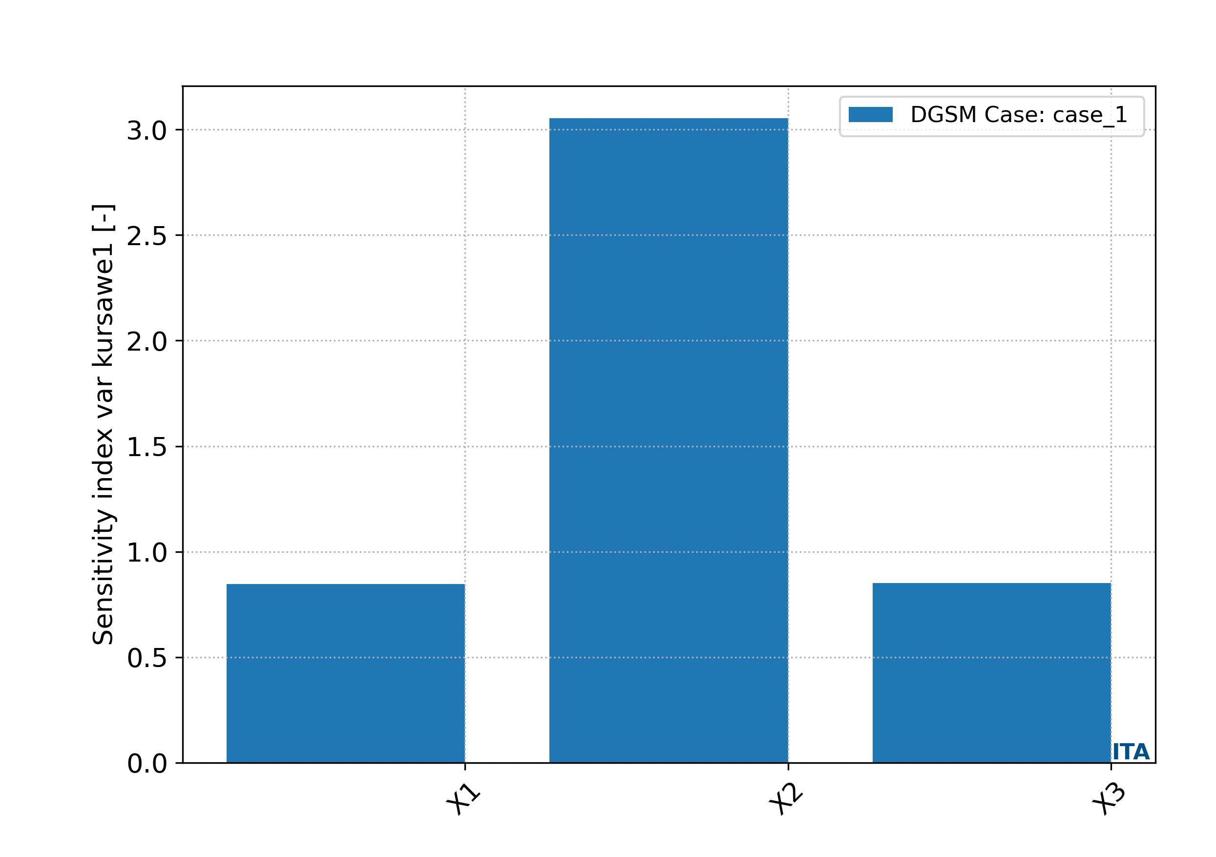
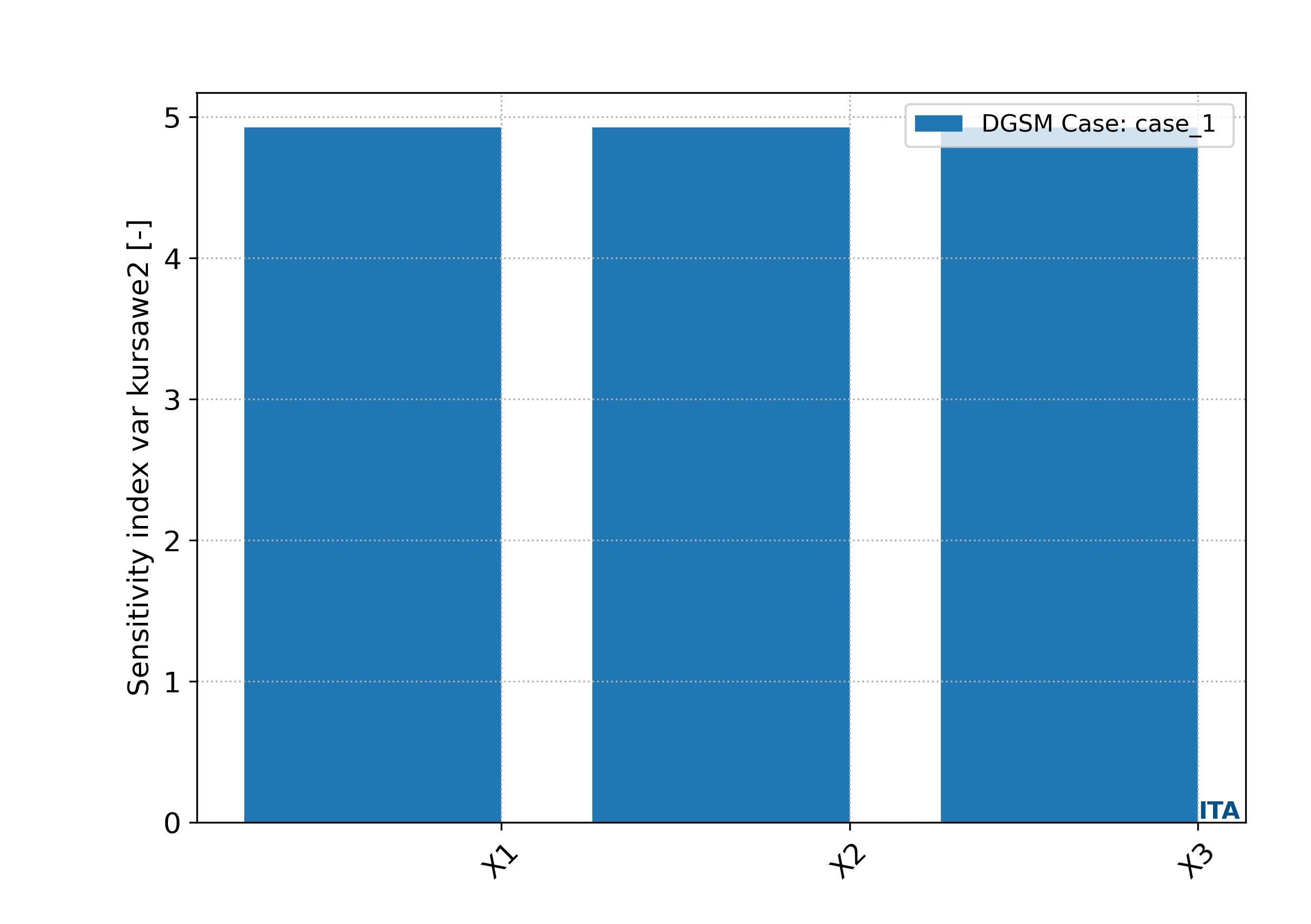
The function output_plts_sensitivity() generates several plots showing the DOEX variables correlation and a summary of the sensitivity analysis. For example this can be seen in Fig. 4.4.1 and Fig. 4.4.2. These plots are located in the output folder.

Fig. 4.4.1 Sensitivity bar plot for case_1, Kursawe function 1. Tutorial A04

Fig. 4.4.2 Sensitivity bar plot for case_1, Kursawe function 2. Tutorial A04

The function run_metamodel_construction() is included in the code to execute the routines related with the metamodeling construction of the DOEY as function of the DOEX data. This functions allows to choose different metamodeling schemas. This schemas perform a robust metamodeling search and find to determine the most adequate metamodeling ML model. Once the ML metamodel is determined allows to predict any data in the ranges of the DOEX and DOEY training values.

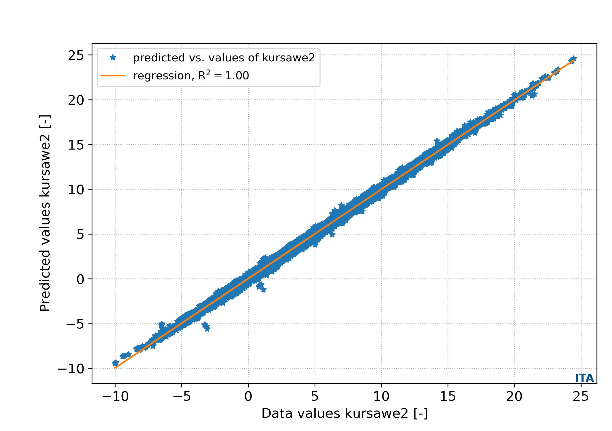
The function output_plts_models_residuals_plot() plots the residual values of the ML metamodel DOEY predictions in comparison with the ground truth DOEY values showing the regression score between the data and the predictions. An example can be seen in Fig. 4.4.7 and Fig. 4.4.8.

In addition, the function output_plts_models_XYZ() plot all the combinations of XYZ plots showing the prediction surfaces constructed using the ML metamodel. An example can be seen in Fig. 4.4.3, Fig. 4.4.4, Fig. 4.4.5, Fig. 4.4.6 and Fig. 4.3.2.

Fig. 4.4.3 Metamodels surface of variable X1 versus X2 versus kursawe1 in case_1. Tutorial A04

Fig. 4.4.4 Metamodels surface of variable X1 versus X3 versus kursawe1 in case_1. Tutorial A04

Fig. 4.4.5 Metamodels surface of variable X2 versus X3 versus kursawe1 in case_1. Tutorial A04

Fig. 4.4.6 Metamodels surface of variable X1 versus X2 versus kursawe2 in case_1. Tutorial A04

Fig. 4.4.7 Metamodels residual plot Kursawe function 1 values versus predictions in case_1. Tutorial A04

Fig. 4.4.8 Metamodels residual plot Kursawe function 2 values versus predictions in case_1. Tutorial A04

4.5. Tutorial case A05: “Sensitivity analysis and metamodeling of a damped oscillator”

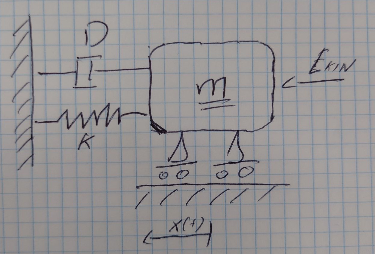
In this tutorial are described the construction of the model, sensitivity analysis and metamodels, as well as the default plotting of them. For this purpose is used the DOE design and sensitivity analysis for a coupled function described in the previous tutorial case as a base line. The damped oscillator is define by a mass paramter \(m\), a spring constant \(k\) and a damping factor \(D\) (see Fig. 4.5.1) drive by a kinetical energy \(E_{kin}\). The damped oscillator is driven by the following equations,

\begin{equation} \begin{cases} \ddot{x} + 2 \cdot D \cdot w_0 \cdot \dot{x} + w_0^2 \cdot x = 0 \quad \quad Differential \ equation \ of \ movement \\ E_{kin} = \frac{m \cdot v^2_0}{2}, \quad x_0=0 \quad \quad Initial \ conditions \\ x(t) = e^{-D \cdot w_0 \cdot t} \cdot \frac{v_0}{w} \cdot sin(w \cdot t) \quad \quad Solution \ eq. \ x(t) \ dependant \ on \ the \ time \\ w_0 = \sqrt{k/m} \quad w = w_0 \sqrt{1-D^2} \quad \quad Natural \ frequency, \ damped \ and \ non-damped \end{cases} \end{equation}

Fig. 4.5.1 Damped oscillator diagram. Tutorial A05

The input and output variable for each of the analysis cases are define in the problem definition spreadsheet file (Download: Problem definition spreadsheet file).

The analysis is performed with pymetamodels based on a basic analysis script as follows in test_analysis.py,

Listing 4.5.1 Damped oscillator test analysis. Sensitivity analysis

#!/usr/bin/env python3

## Analytical model,
##

import os, sys, random
import numpy as np
import gc

import pymetamodels
import damped_model as model_obj

class analysis(object):

    """

    .. _model_damped_oscillator_metamodel:

    **Synopsis:**
        * Analysis framework with pymetamodels
        * Damped oscillator tutorial

    """

    def __init__(self):
        
        ## Initial variables
        self.name = "damped_oscillator"
        self.folder_script = os.path.dirname(os.path.realpath(__file__))

        self.folder_path_inputs = self.folder_script

        self.folder_path_outputs = os.path.join(os.path.join(os.path.join(self.folder_script, os.pardir), "_examples_raw"),self.name + "_out")
        if not os.path.exists(self.folder_path_outputs): os.makedirs(self.folder_path_outputs)

        self.file_name_inputs = r"configuration_spreadsheet"
        self.file_name_outputs = r"outputs"

        ## Initialise 
        self.mita = pymetamodels.load()
        self.mita.logging_start(self.folder_path_outputs)          

    def run_model(self):

        ## Inputs load
        folder_path = self.folder_path_inputs
        file_name = self.file_name_inputs
        self.mita.read_xls_case(folder_path, file_name, sheet="cases", col_start = 0, row_start = 1, tit_row = 0 )

        ## Sampling
        for case in self.mita.keys():

            ## Run samplimg cases
            self.mita.run_sampling_routine(case)

            ## Run / Load model
            self.model_iteration(case, model_obj)

            ## Sensitivity analysis
            self.mita.run_sensitivity_analisis(case)

            ## Metamodeling construction
            #self.mita.run_metamodel_construction(case, scheme = "general")
            self.mita.run_metamodel_construction(case, scheme = "general_fast")

        ##
        self.mita.run_sensitivity_normalization()

        ## Ploting and others
        for case in self.mita.keys():

            ## Plots cross varible relation in the sensitivity analysis
            self.mita.output_plts_sensitivity(self.folder_path_outputs, case)

            ## Plots showing the model DOEX and DOEY variables relationship 2D XY
            self.mita.output_plts_models_XY(self.folder_path_outputs, case)

            ## Residual values plots
            self.mita.output_plts_models_residuals_plot(self.folder_path_outputs, case)

            ## Plots showing the model DOEX and DOEY variables relationship 3D XYZ
            self.mita.output_plts_models_XYZ(self.folder_path_outputs, case, scatter = False)

        ## Output variables save
        folder_path = self.folder_path_outputs
        file_name = self.file_name_outputs
        out_path = self.mita.output_xls(folder_path, file_name, col_start = 0, tit_row = 0)

    def model_iteration(self, case, _model_obj):

        ## Model iteration to generate Y doe output values
        doeX = self.mita.doeX(case)
        doeY = self.mita.doeY(case)
        vars_in = self.mita.vars_parameter_matrix(case)
        case_dict = self.mita.case[case]
        samples = len(doeX[list(doeX.keys())[0]])

        for ii in range(0, samples):

            obj_model = _model_obj.model_obj()

            # initialize dictionaries
            obj_model.doeX = doeX
            obj_model.doeY = doeY
            obj_model.case_dict = case_dict
            obj_model.ii = ii
            obj_model.vars_in = vars_in

            # add variables as atributes
            for key in obj_model.doeX.keys():
                setattr(obj_model, key, obj_model.doeX[key][obj_model.ii])

            # run the model for ii sample
            obj_model.run_model()

if __name__ == "__main__":

    analysis = analysis()

    analysis.run_model()

The analysis frameworks iterates the model defined in a secondary file as follows in damped_oscillator.py,

Listing 4.5.2 Damped oscillator model code block. Sensitivity analysis

#!/usr/bin/env python3

## damped oscillator
##

import os, sys, random
import numpy as np
from math import exp, pow, sqrt, sin

class model_obj(object):

    """

    .. _model_id_001_damped_oscillator:

    **Damped oscillator functions model**

    :platform: Unix, Windows
    :synopsis: Damped oscillator
    :author:

    :Dependences:

    """

    def __init__(self):

        ## Initial variables
        self.doeX = None
        self.doeY = None
        self.case_dict = None
        self.ii = None

    def run_model(self):

        # variables
        m = self.doeX["m"][self.ii] #kg [0.1,5.0]
        k = self.doeX["k"][self.ii] # N/m [20,50]

        D = self.doeX["D"][self.ii]
        Ekin = self.doeX["E_{kin}"][self.ii] #10 [Nm]

        # calculations
        omega_0 = (k/m)**0.5 #w_0
        omega = omega_0 * (1-(D**2.))**0.5 #w
        v_0 = ((2*Ekin)/m)**0.5

        num_steps = 101
        t_max =  10
        t_observe = 5 # x(t>5) -> min

        # time serie
        t_serie = []
        for ii in range(0,num_steps):
            t_serie.append(t_observe+ii*float(t_max-t_observe)/num_steps)

        # ------------------------- #
        #   Results
        # ------------------------- #
        # time serie values
        x_serie = []
        for ii in range(0,num_steps):
            tt_serie = t_serie[ii]
            xx_serie = exp(-1*D*omega_0*tt_serie)*(v_0/omega)*sin(omega*tt_serie)
            x_serie.append(xx_serie)

        # find max value
        ref = None
        for ii in range(0,num_steps):
            if ref is None: ref = abs(x_serie[ii])
            if abs(x_serie[ii]) >= ref: ref = abs(x_serie[ii])

        x_max = ref

        w_damped = omega_0 * (1-(D**2.))**0.5

        # outputs
        self.doeY["x_{max}"][self.ii] = x_max
        self.doeY["w_{damped}"][self.ii] = w_damped

The function output_plts_sensitivity() generates several plots showing the DOEX variables correlation and a summary of the sensitivity analysis. For example this can be seen in Fig. 4.5.2 and Fig. 4.5.3. These plots are located in the output folder.

Fig. 4.5.2 Sensitivity bar plot for case_2, :math:` x_{max}`. Tutorial A05

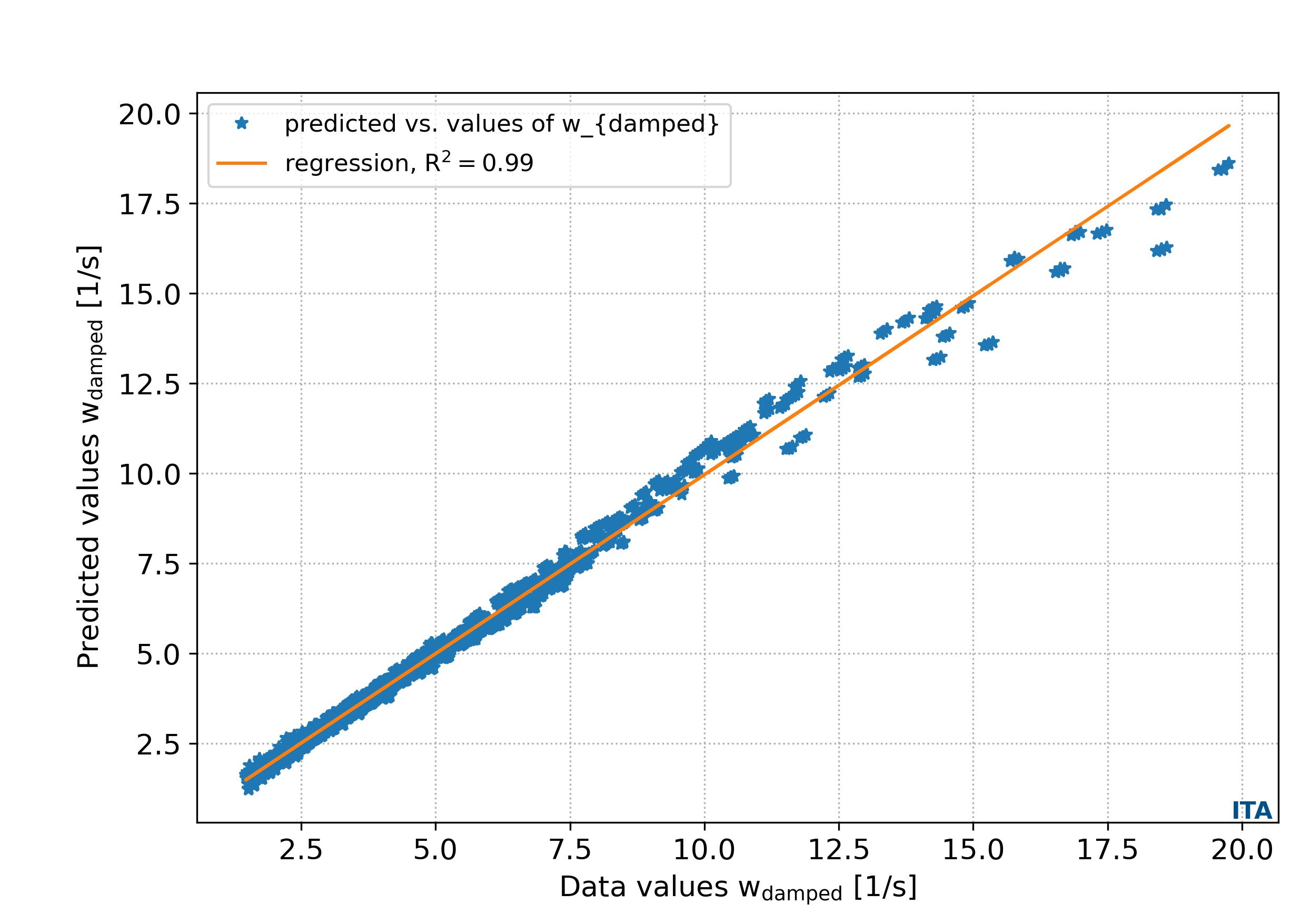
Fig. 4.5.3 Sensitivity bar plot for case_1, \(w_{damped}\). Tutorial A05

The function run_metamodel_construction() is included in the code to execute the routines related with the metamodeling construction of the DOEY as function of the DOEX data. This functions allows to choose different metamodeling schemas. This schemas perform a robust metamodeling search and find to determine the most adequate metamodeling ML model. Once the ML metamodel is determined allows to predict any data in the ranges of the DOEX and DOEY training values.

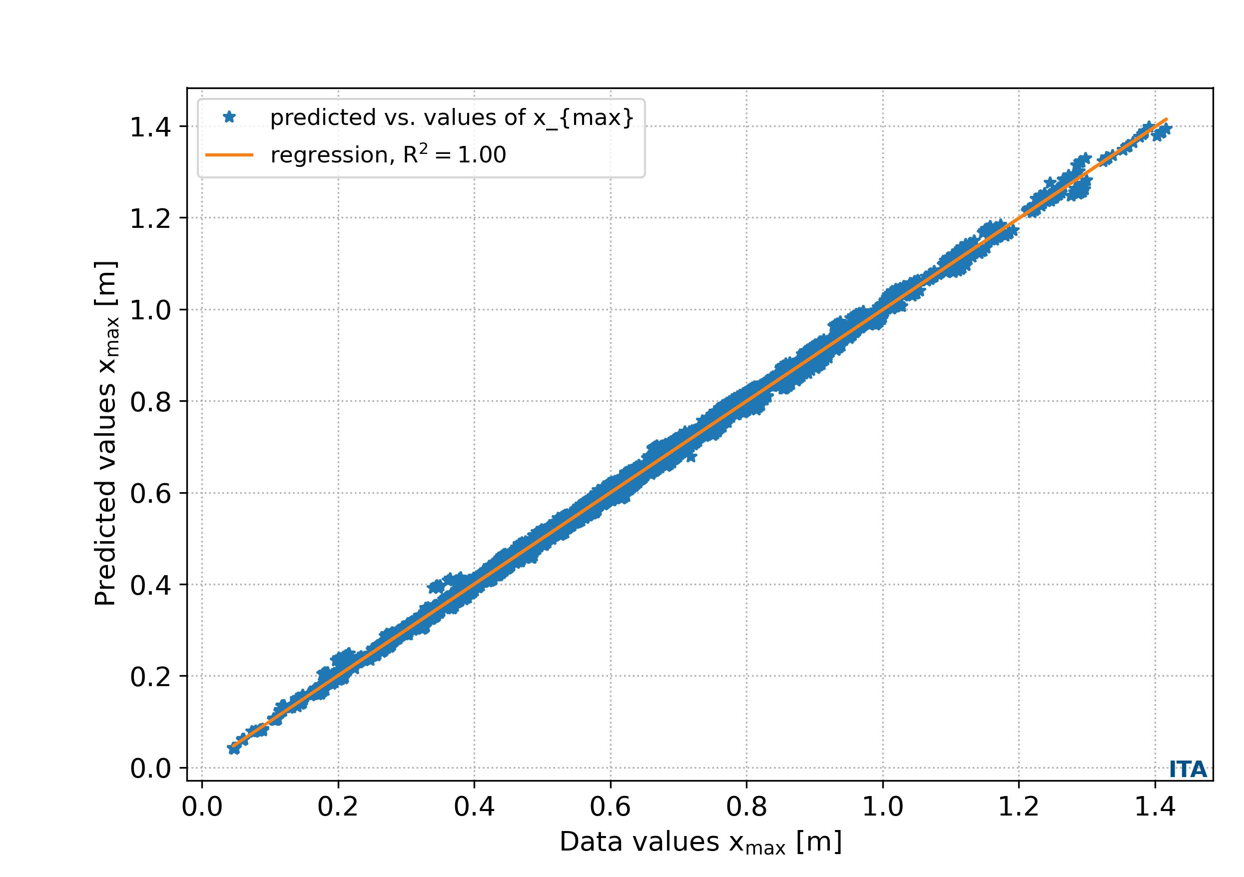
The function output_plts_models_residuals_plot() plots the residual values of the ML metamodel DOEY predictions in comparison with the ground truth DOEY values showing the regression score between the data and the predictions. An example can be seen in Fig. 4.4.7 and Fig. 4.4.8.

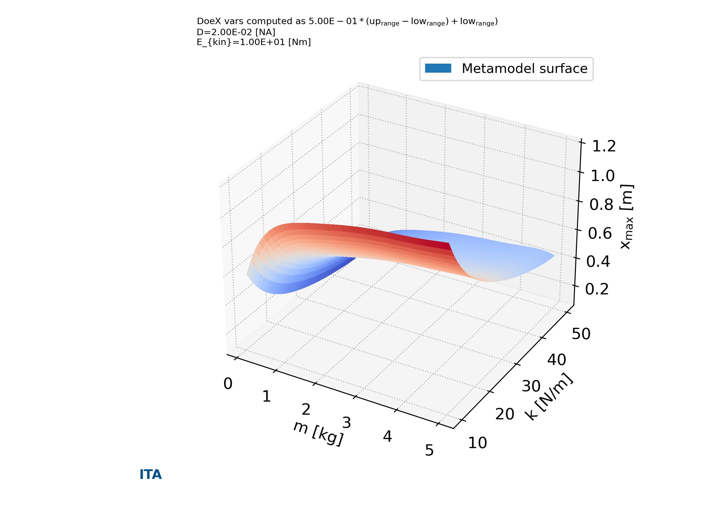
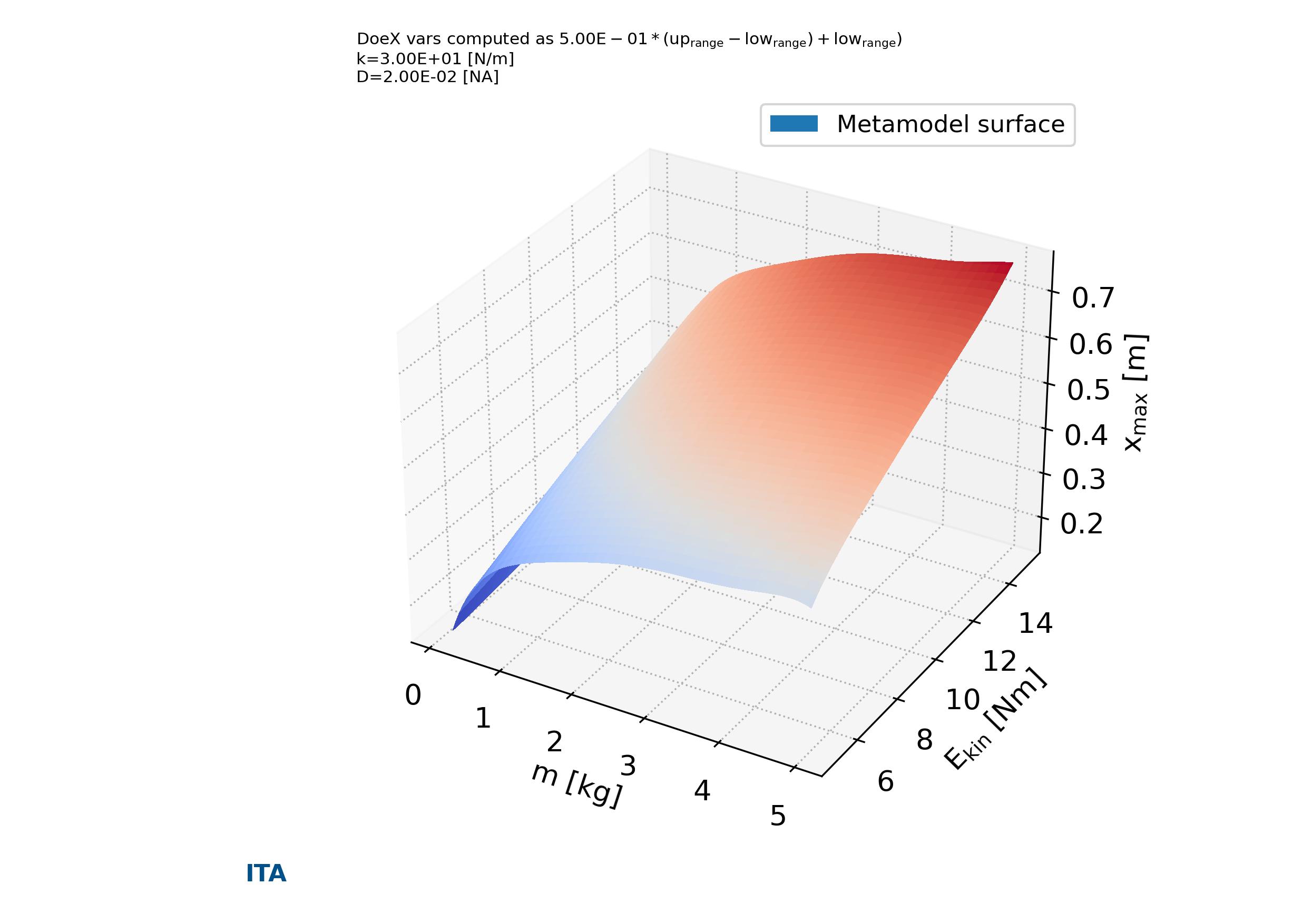
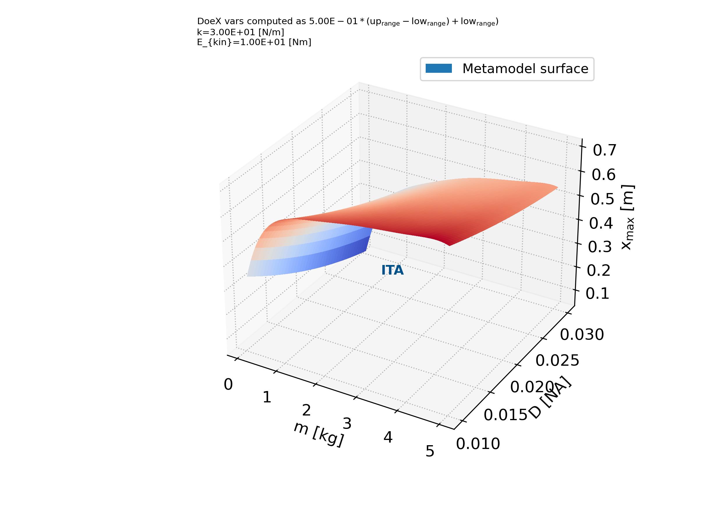
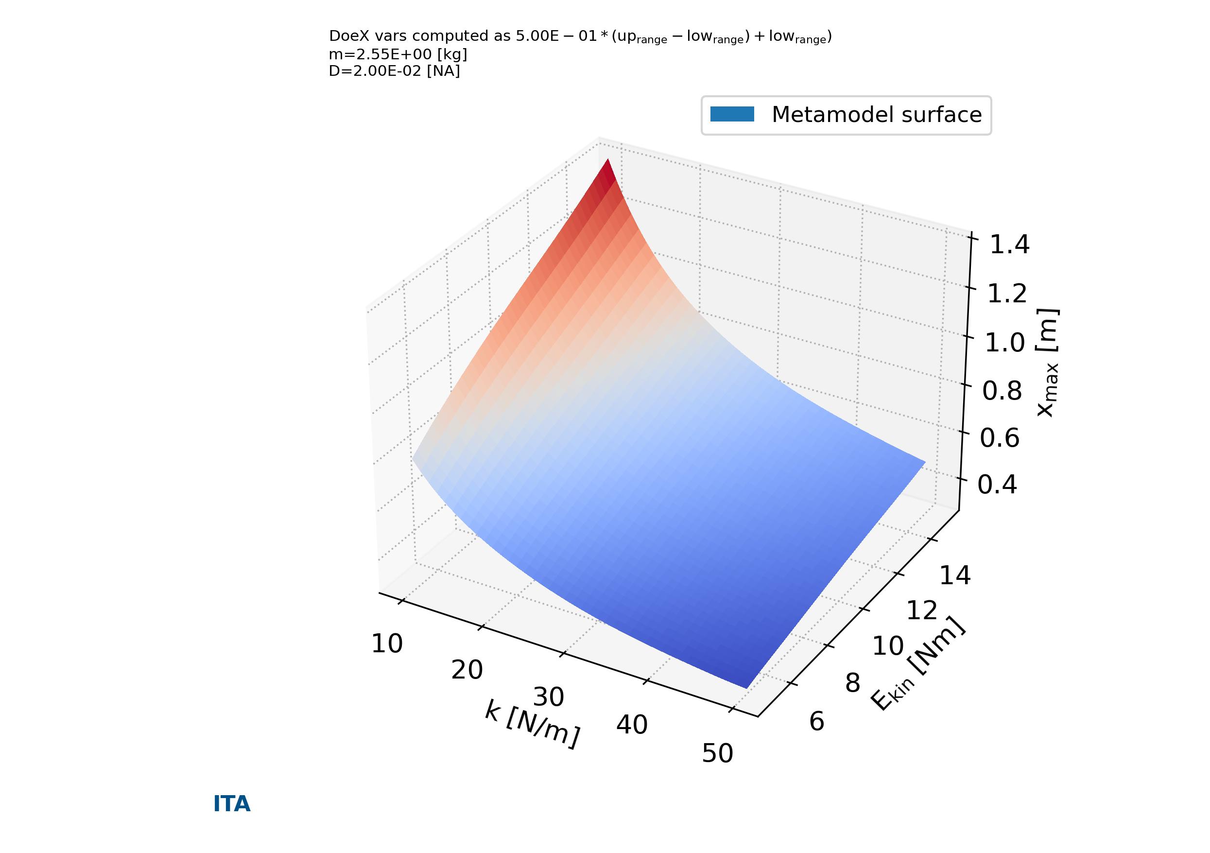
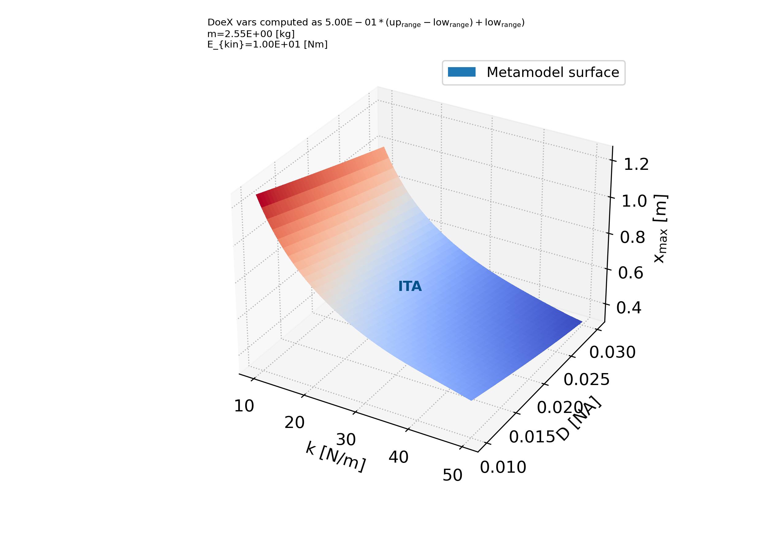
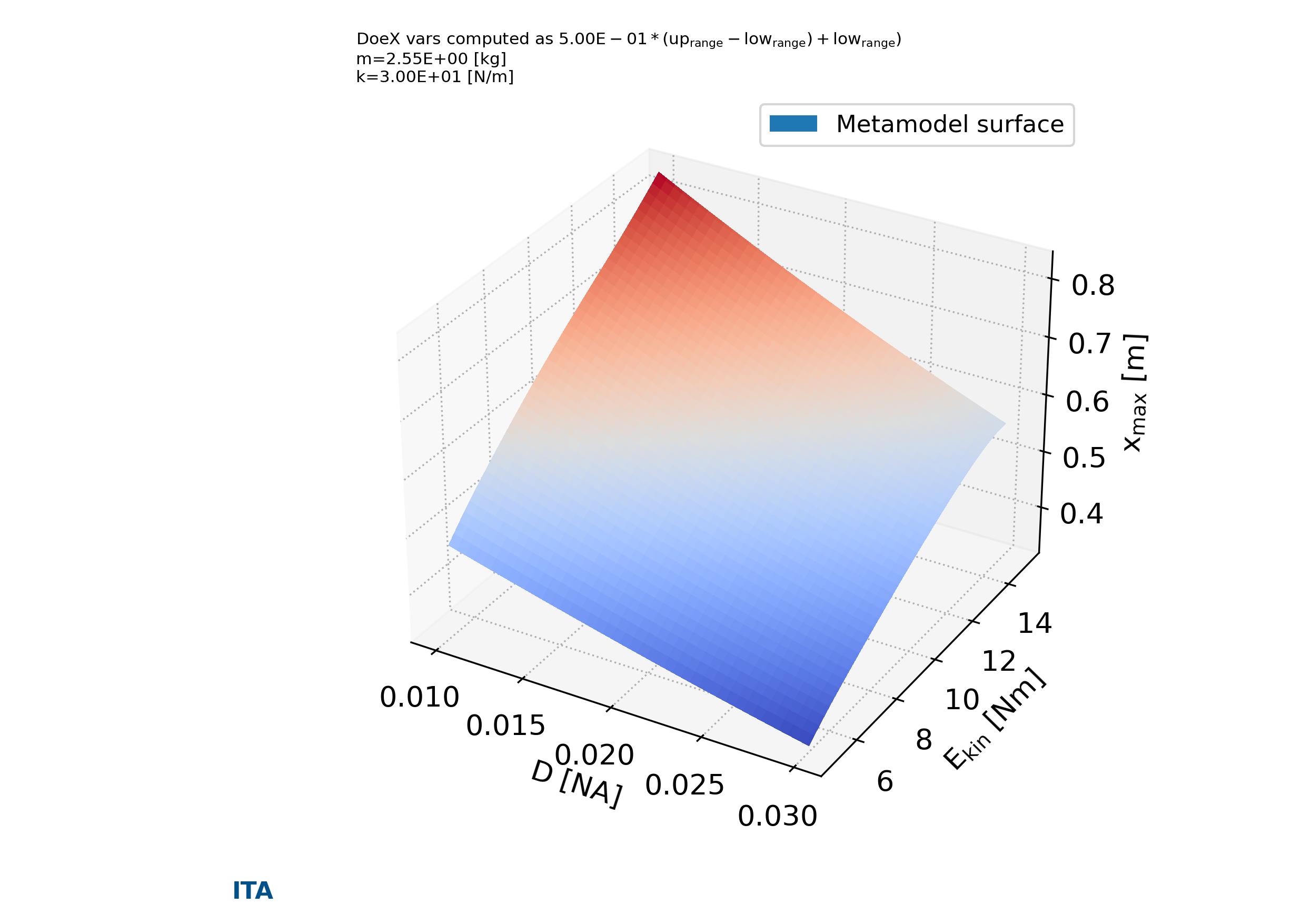
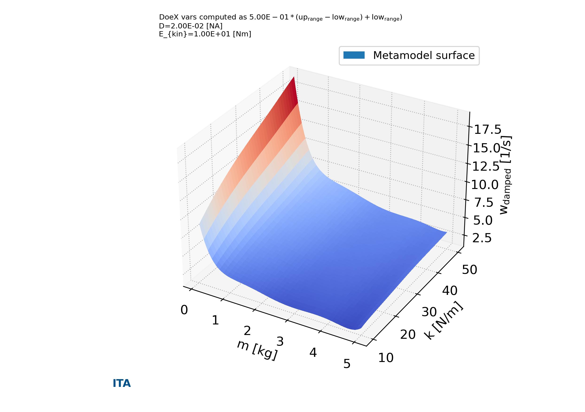
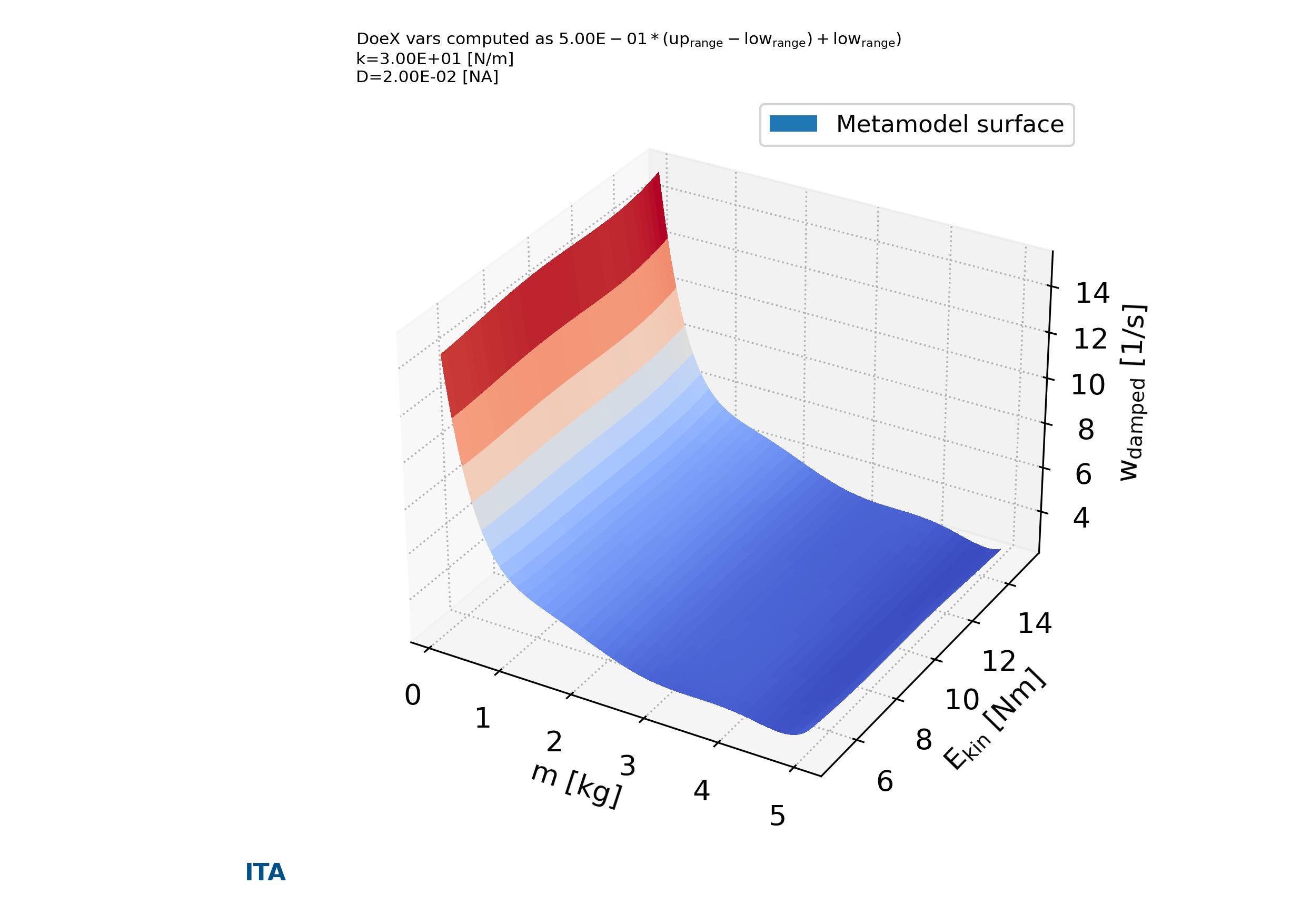
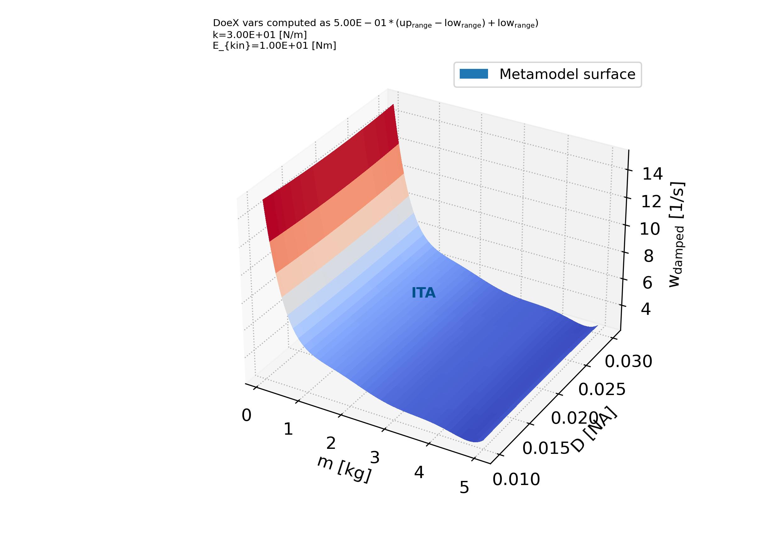
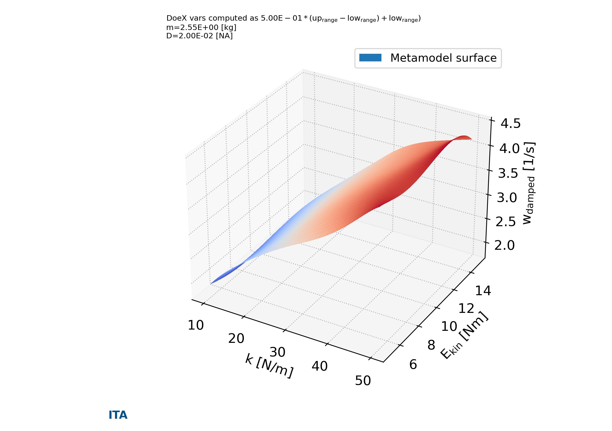
In addition, the function output_plts_models_XYZ() plot all the combinations of XYZ plots showing the prediction surfaces constructed using the ML metamodel. An example can be seen from Fig. 4.5.4 to Fig. 4.5.13.

Fig. 4.5.4 Metamodels surface of variable \(m\) versus \(k\) versus \(x_{max}\) in case_2. Tutorial A05

Fig. 4.5.5 Metamodels surface of variable \(m\) versus \(E_{kin}\) versus \(x_{max}\) in case_2. Tutorial A05

Fig. 4.5.6 Metamodels surface of variable \(m\) versus \(D\) versus \(x_{max}\) in case_2. Tutorial A05

Fig. 4.5.7 Metamodels surface of variable \(k\) versus \(E_{kin}\) versus \(x_{max}\) in case_2. Tutorial A05

Fig. 4.5.8 Metamodels surface of variable \(k\) versus \(D\) versus \(x_{max}\) in case_2. Tutorial A05

Fig. 4.5.9 Metamodels surface of variable \(E_{kin}\) versus \(D\) versus \(x_{max}\) in case_2. Tutorial A05

Fig. 4.5.10 Metamodels surface of variable \(m\) versus \(k\) versus \(w_{damped}\) in case_2. Tutorial A05

Fig. 4.5.11 Metamodels surface of variable \(m\) versus \(E_{kin}\) versus \(w_{damped}\) in case_2. Tutorial A05

Fig. 4.5.12 Metamodels surface of variable \(m\) versus \(D\) versus \(w_{damped}\) in case_2. Tutorial A05

Fig. 4.5.13 Metamodels surface of variable \(k\) versus \(E_{kin}\) versus \(w_{damped}\) in case_2. Tutorial A05

4.6. Tutorial case A06: “Minimization of the Kursawe Functions”

In this tutorial is described the extension of tutorial A04 Section 4.4 regarding the Kursawe Functions with the minimization of one of the Kursawe functions according a non linear constrain. This problem is described in Eq.4.4.1.

\begin{equation} optimization \begin{cases} min[f_{2}(x)] \\ constrains: \\ \quad \quad f_{1}(x) \leqslant -14.5 \end{cases} \end{equation}

The input and output variable for each of the analysis cases are define in the problem definition spreadsheet file (Download: Problem definition spreadsheet file).

The same model as in tutorial A04 (see Section 4.4) is used. The analysis is performed with pymetamodels based on a basic analysis script as follows in test_analysis.py (see Listing 4.6.1).

Apart of the sensitivity analysis and metamodeling construction carried out in tutorial A04. The optimization routine is call with the function run_optimization_problem() using a “general_fast” schema approach. The optimization problem is solve resulting in Eq.4.6.2.

\begin{equation} \begin{cases} optimization\\ result \end{cases} \begin{cases} min[f_{2}(x)] = -7.5074 \\ constrains: \\ \quad \quad f_{1}(x) \leqslant -14.5 \\ where, \\ f_{1}(x)=-14.5000 \\ [X_1, X_2, X_3] = [-1.30575601, -0.87599992, -1.33713208] \end{cases} \end{equation}

Listing 4.6.1 Kursawe Functions test analysis. Minimization of the Kursawe Functions

#!/usr/bin/env python3

## Analytical model,
##

import os, sys, random
import numpy as np
import gc

import pymetamodels
import kursawe_model as model_obj

class analysis(object):

    """

    .. _model_kursawe_model_optimize:

    **Synopsis:**
        * Analysis framework with pymetamodels
        * Coupled function tutorial

    """

    def __init__(self):
        
        ## Initial variables
        self.name = "kuwase_optimize"
        self.folder_script = os.path.dirname(os.path.realpath(__file__))

        self.folder_path_inputs = self.folder_script

        self.folder_path_outputs = os.path.join(os.path.join(os.path.join(self.folder_script, os.pardir), "_examples_raw"),self.name + "_out")
        if not os.path.exists(self.folder_path_outputs): os.makedirs(self.folder_path_outputs)

        self.file_name_inputs = r"configuration_spreadsheet"
        self.file_name_outputs = r"outputs"

        ## Initialise 
        self.mita = pymetamodels.load()
        self.mita.logging_start(self.folder_path_outputs)          

    def run_model(self):

        ## Inputs load
        folder_path = self.folder_path_inputs
        file_name = self.file_name_inputs
        self.mita.read_xls_case(folder_path, file_name, sheet="cases", col_start = 0, row_start = 1, tit_row = 0 )

        ## Sampling
        for case in self.mita.keys():

            ## Run samplimg cases
            self.mita.run_sampling_routine(case)

            ## Run / Load model
            self.model_iteration(case, model_obj)

            ## Sensitivity analysis
            self.mita.run_sensitivity_analisis(case)

            ## Metamodeling construction
            if self.mita.load_metamodel(self.folder_path_outputs, case):
                pass
            else:
                self.mita.run_metamodel_construction(case, scheme = "general_fast")

                ## Save metamodels .metaita
                self.mita.save_metamodel(self.folder_path_outputs, case)

            ## Solve optimization problem
            self.mita.run_optimization_problem(case, scheme = "general_fast", verbose_testing = True)

        ##
        self.mita.run_sensitivity_normalization()

        ## Ploting and others
        for case in self.mita.keys():

            ## Save DOEX and DOEY

            ## Plots cross varible relation in the sensitivity analysis
            self.mita.output_plts_sensitivity(self.folder_path_outputs, case)

            ## Plots showing the model DOEX and DOEY variables relationship 2D XY
            self.mita.output_plts_models_XY(self.folder_path_outputs, case)

            ## Residual values plots
            self.mita.output_plts_models_residuals_plot(self.folder_path_outputs, case)

            ## Plots showing the model DOEX and DOEY variables relationship 3D XYZ
            self.mita.output_plts_models_XYZ(self.folder_path_outputs, case, scatter = False)

        ## Output variables save
        folder_path = self.folder_path_outputs
        file_name = self.file_name_outputs
        out_path = self.mita.output_xls(folder_path, file_name, col_start = 0, tit_row = 0)

    def model_iteration(self, case, _model_obj):

        ## Model iteration to generate Y doe output values
        doeX = self.mita.doeX(case)
        doeY = self.mita.doeY(case)
        vars_in = self.mita.vars_parameter_matrix(case)
        case_dict = self.mita.case[case]
        samples = len(doeX[list(doeX.keys())[0]])

        for ii in range(0, samples):

            obj_model = _model_obj.model_obj()

            # initialize dictionaries
            obj_model.doeX = doeX
            obj_model.doeY = doeY
            obj_model.case_dict = case_dict
            obj_model.ii = ii
            obj_model.vars_in = vars_in

            # add variables as atributes
            for key in obj_model.doeX.keys():
                setattr(obj_model, key, obj_model.doeX[key][obj_model.ii])

            # run the model for ii sample
            obj_model.run_model()

if __name__ == "__main__":

    analysis = analysis()

    analysis.run_model()

4.7. Tutorial case A07: “Calibration of a damped oscillator”

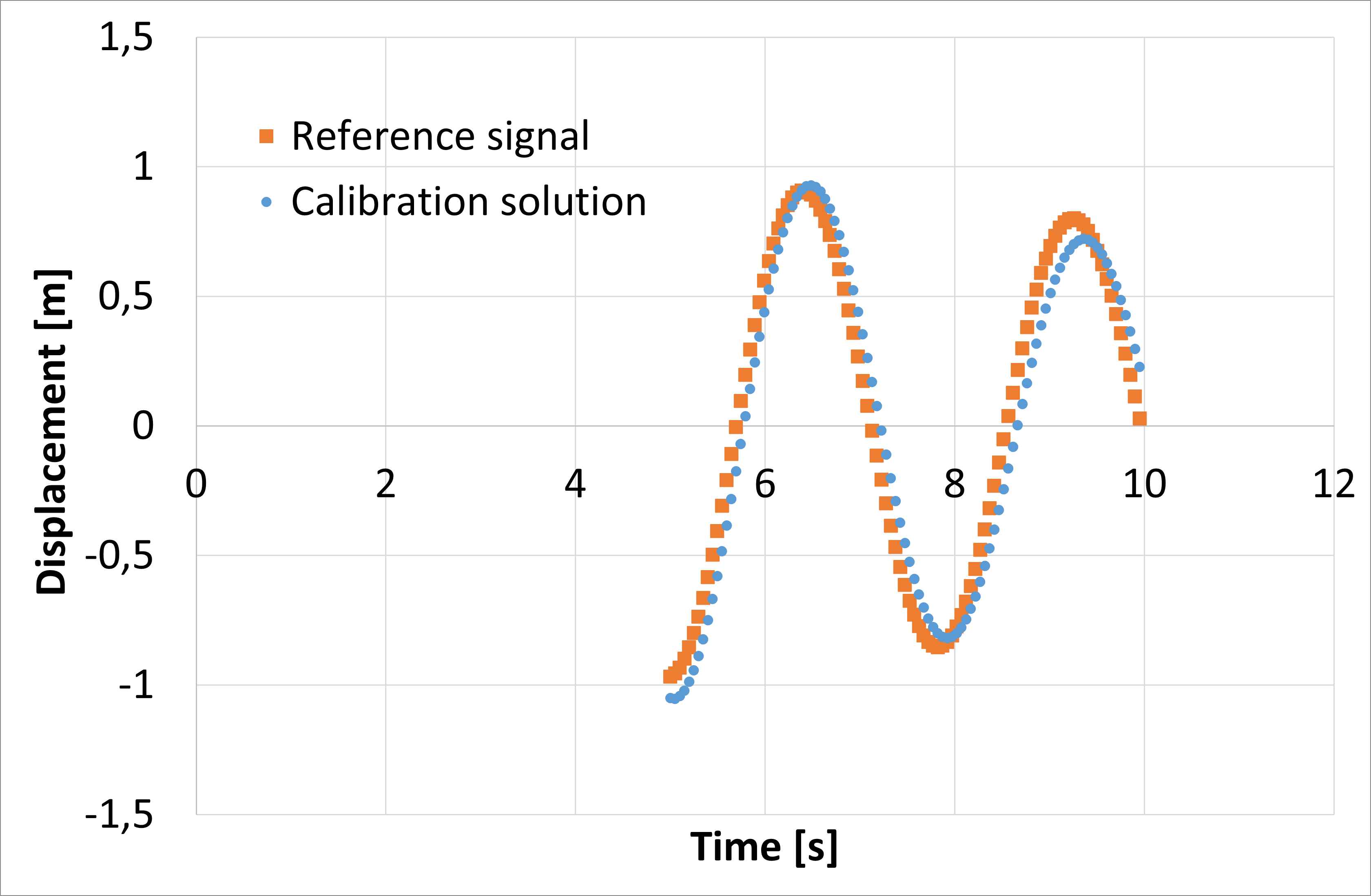
In this tutorial is described the extension of tutorial A05 Section 4.5 regarding a damped oscillator with the calibration of the oscillating system according a given reference signal. This problem is described in Eq.4.7.1.

\begin{equation} \begin{cases} optimization \begin{cases} calibrate[(simulation,reference)] = 0 \\ constrains: \\ \quad \quad w_{damped} \leq 10 \ \text{[1/s]} \\ \quad \quad m \in [0.1, 5.0] \ \text{[kg]} \\ \quad \quad k \in [10, 50] \ \text{[N/m]} \\ \quad \quad D \in [0.01, 0.05] \\ \quad \quad E_{kin} \in [10, 50] \ \text{[Nm]} \\ \end{cases} \\ \end{cases} \end{equation}

The input and output variable for each of the analysis cases are define in the problem definition spreadsheet file (Download: Problem definition spreadsheet file).

The same model as in tutorial A05 (see Section 4.5) is used, with a small modification. The constrain function and the objective function to be minimize as equal to zero has been added (see Listing 4.7.2). In addition the reference signal to be math in the calibration is loaded (Download: Reference signal spreadsheet file) in order to build the objective function.

The analysis is performed with pymetamodels based on a basic analysis script as follows in test_analysis.py (see Listing 4.7.1). Apart of the sensitivity analysis and metamodeling construction carried out in tutorial A05. The optimization routine is call with the function run_optimization_problem() using a “general_fast” schema approach.

The calibration problem is solve resulting in Eq.4.7.2. When the reference and simulation signal for the aforementioned values are compared in Fig. 4.7.1 showing a good agreement for the calibration solution values.

\begin{equation} \begin{cases} optimization \begin{cases} calibrate[(simulation,reference)] = -8.7e-04 \\ constrains: \\ \quad \quad x_{max} = 4.45555556 \ \text{[m]} \\ \quad \quad w_{damped} = 2.02715485 \ \text{[1/s]} \\ \quad \quad m = 3.775 \ \text{[kg]} \\ \quad \quad k = 15. \ \text{[N/m]} \\ \quad \quad D = 0.04 \\ \quad \quad E_{kin} = 10. \ \text{[Nm]} \\ \end{cases} \\ \end{cases} \end{equation}

Fig. 4.7.1 Damped oscillator calibration. Tutorial A07

Listing 4.7.1 Damped oscillator test analysis. Calibration analysis

#!/usr/bin/env python3

## Analytical model,
##

import os, sys, random
import numpy as np
import gc

import pymetamodels
import damped_model as model_obj

class analysis(object):

    """

    .. _model_damped_oscillator_optimize:

    **Synopsis:**
        * Analysis framework with pymetamodels
        * Coupled function tutorial

    """

    def __init__(self):

        ## Initial variables
        self.name = "damped_oscillator_op"
        self.folder_script = os.path.dirname(os.path.realpath(__file__))

        self.folder_path_inputs = self.folder_script

        self.folder_path_outputs = os.path.join(os.path.join(os.path.join(self.folder_script, os.pardir), "_examples_raw"),self.name + "_out")
        if not os.path.exists(self.folder_path_outputs): os.makedirs(self.folder_path_outputs)

        self.file_name_inputs = r"configuration_spreadsheet"
        self.file_name_outputs = r"outputs"

        ## Initialise 
        self.mita = pymetamodels.load()
        self.mita.logging_start(self.folder_path_outputs)          

    def run_model(self):

        ## Inputs load
        folder_path = self.folder_path_inputs
        file_name = self.file_name_inputs
        self.mita.read_xls_case(folder_path, file_name, sheet="cases", col_start = 0, row_start = 1, tit_row = 0 )

        ## Sampling
        for case in self.mita.keys():

            ## Run samplimg cases
            self.mita.run_sampling_routine(case)

            ## Run / Load model
            self.model_iteration(case, model_obj)

            ## Sensitivity analysis
            self.mita.run_sensitivity_analisis(case)

            ## Metamodeling construction
            if self.mita.load_metamodel(self.folder_path_outputs, case):
                pass
            else:
                #self.mita.run_metamodel_construction(case, scheme = "general_fast")
                self.mita.run_metamodel_construction(case, scheme = "neural")

                ## Save metamodels .metaita
                self.mita.save_metamodel(self.folder_path_outputs, case)

            ## Solve optimization problem
            if self.mita.load_optimization(self.folder_path_outputs, case):
                pass
            else:
                max_size_grid_methods = 5e4
                self.mita.run_optimization_problem(case, scheme = "general_fast", max_size_grid_methods = max_size_grid_methods, verbose_testing = False)

                ## Save optimization .optita
                self.mita.save_optimization(self.folder_path_outputs, case)

        ##
        self.mita.run_sensitivity_normalization()

        ## Ploting and others
        for case in self.mita.keys():

            ## Save DOEX and DOEY

            ## Plots cross varible relation in the sensitivity analysis
            self.mita.output_plts_sensitivity(self.folder_path_outputs, case)

            ## Plots showing the model DOEX and DOEY variables relationship 2D XY
            self.mita.output_plts_models_XY(self.folder_path_outputs, case)

            ## Residual values plots
            self.mita.output_plts_models_residuals_plot(self.folder_path_outputs, case)

            ## Plots showing the model DOEX and DOEY variables relationship 3D XYZ
            self.mita.output_plts_models_XYZ(self.folder_path_outputs, case, scatter = False)

        ## Output variables save
        folder_path = self.folder_path_outputs
        file_name = self.file_name_outputs
        out_path = self.mita.output_xls(folder_path, file_name, col_start = 0, tit_row = 0)

    def model_iteration(self, case, _model_obj):

        ## Model iteration to generate Y doe output values
        doeX = self.mita.doeX(case)
        doeY = self.mita.doeY(case)
        vars_in = self.mita.vars_parameter_matrix(case)
        case_dict = self.mita.case[case]
        samples = len(doeX[list(doeX.keys())[0]])

        for ii in range(0, samples):

            obj_model = _model_obj.model_obj()

            # initialize dictionaries
            obj_model.doeX = doeX
            obj_model.doeY = doeY
            obj_model.case_dict = case_dict
            obj_model.ii = ii
            obj_model.vars_in = vars_in

            # add variables as atributes
            for key in obj_model.doeX.keys():
                setattr(obj_model, key, obj_model.doeX[key][obj_model.ii])

            # run the model for ii sample
            obj_model.run_model()

if __name__ == "__main__":

    analysis = analysis()

    analysis.run_model()

Listing 4.7.2 Damped oscillator model code block. Calibration analysis

#!/usr/bin/env python3

## damped oscillator
##

import os, sys, random
import numpy as np
from math import exp, pow, sqrt, sin
import pymetamodels

class model_obj(object):

    """

    .. _model_id_001_damped_oscillator_op:

    **Damped oscillator functions model**

    :platform: Unix, Windows
    :synopsis: Damped oscillator
    :author:

    :Dependences:

    """

    def __init__(self):

        ## Initial variables
        self.doeX = None
        self.doeY = None
        self.case_dict = None
        self.ii = None

    def run_model(self):

        # variables
        m = self.doeX["m"][self.ii] #kg [0.1,5.0]
        k = self.doeX["k"][self.ii] # N/m [20,50]

        D = self.doeX["D"][self.ii]
        Ekin = self.doeX["E_{kin}"][self.ii] #10 [Nm]

        # calculations
        omega_0 = (k/m)**0.5 #w_0
        omega = omega_0 * (1-(D**2.))**0.5 #w
        v_0 = ((2*Ekin)/m)**0.5

        num_steps = 101
        t_max =  10
        t_observe = 5 # x(t>5) -> min

        # time serie
        t_serie = []
        for ii in range(0,num_steps):
            t_serie.append(t_observe+ii*float(t_max-t_observe)/num_steps)

        # ------------------------- #
        #   Results
        # ------------------------- #
        # time serie values
        x_serie = []
        for ii in range(0,num_steps):
            tt_serie = t_serie[ii]
            xx_serie = exp(-1*D*omega_0*tt_serie)*(v_0/omega)*sin(omega*tt_serie)
            x_serie.append(xx_serie)

        # find max value
        ref = None
        for ii in range(0,num_steps):
            if ref is None: ref = abs(x_serie[ii])
            if abs(x_serie[ii]) >= ref: ref = abs(x_serie[ii])

        x_max = ref

        w_damped = omega_0 * (1-(D**2.))**0.5

        # compute simulation - reference absolute value
        mmita = pymetamodels.load()
        file_name = "reference.csv"
        path_out = os.path.dirname(os.path.realpath(__file__))
        reference, units = mmita.read_table_csv_channels(file_name, path_out, units_chn = False)
        x_serie = np.asarray(x_serie,dtype=np.dtype('float64'))
        reference = np.asarray(reference["disp"],dtype=np.dtype('float64'))
        if len(x_serie) - len(reference) != 0: error

        # outputs
        self.doeY["x_{max}"][self.ii] = x_max
        self.doeY["w_{damped}"][self.ii] = w_damped
        self.doeY["cons-w_{damped}"][self.ii] = 10.-w_damped
        self.doeY["min-obj"][self.ii] = np.sum(np.square(x_serie-reference))

4.8. Tutorial case A08: “Building the configuration spreadsheet programatically”

Based in the tutorial related with the coupled function, in this tutorial is described how to build the configuration spreadsheet programatically using the objconf(). The analysis includes the sampling, metamodeling and optimization routines.

The code to print the data structure objects are described in the script as follows in test_analysis.py,

Listing 4.8.1 Coupled function test analysis. Objconf()

## Analytical model,
##

import os, sys, random
import numpy as np
import gc

import pymetamodels
import coupled_function_model as model_obj

class analysis(object):

    """

    .. _model_coupled_function_obj_conf:

    **Synopsis:**
        * Analysis framework with pymetamodels
        * Coupled function tutorial

    """

    def __init__(self):

        ## Initial variables
        self.name = "coupled_function_obj_conf"
        self.folder_script = os.path.dirname(os.path.realpath(__file__))

        self.folder_path_inputs = self.folder_script

        self.folder_path_outputs = os.path.join(os.path.join(os.path.join(self.folder_script, os.pardir), "_examples_raw"),self.name + "_out")
        if not os.path.exists(self.folder_path_outputs): os.makedirs(self.folder_path_outputs)

        self.file_name_inputs = r"configuration_spreadsheet"
        self.file_name_outputs = r"outputs"

        ## Initialise 
        self.mita = pymetamodels.load()
        self.mita.logging_start(self.folder_path_outputs)

    def run_model(self):

        ## Build programatically configuration sheet
        _conf = self.mita.objconf()
        _conf.start(self.folder_path_inputs, self.file_name_inputs)

        _conf.add_case("case_1","case_1_vars_sensi","case_out",1024,"DGSM")
        _conf.add_case("case_2","case_1_vars_sensi","case_out_2",256,"DGSM")

        _conf.add_vars_sheet_variable("case_1_vars_sensi","X1", 1, -3.14, 3.14, "unif", True, 5/100., "[-]", "X1")
        _conf.add_vars_sheet_variable("case_1_vars_sensi","X2", 1, -3.14, 3.14, "unif", True, 5/100., "[-]", "X2")
        _conf.add_vars_sheet_variable("case_1_vars_sensi","X3", 1, -3.14, 3.14, "unif", True, 5/100., "[-]", "X3")
        _conf.add_vars_sheet_variable("case_1_vars_sensi","X4", 1, -3.14, 3.14, "unif", True, 5/100., "[-]", "X4")
        _conf.add_vars_sheet_variable("case_1_vars_sensi","X5", 1, -3.14, 3.14, "unif", True, 5/100., "[-]", "X5")
        _conf.add_vars_sheet_variable("case_1_vars_sensi","cte", 1., 1., 1., "unif", False, 5/100., "[-]", "cte")

        _conf.add_output_sheet("case_out", "Y", None, "m^3", False, True, False, False, False, "function output")
        _conf.add_output_sheet("case_out_2", "Y", None, "m^3", False, True, False, False, False, "function output")
        _conf.add_output_sheet("case_out_2", "Y2", None, "m^3", False, False, False, False, False, "function output")

        _conf.save_conf()

        ## Inputs load
        self.mita.read_xls_case(self.folder_path_inputs, self.file_name_inputs)

        ## Sampling, metamodeling and optimization
        for case in self.mita.keys():

            ## Run samplimg cases
            self.mita.run_sampling_routine(case)

            ## Run / Load model
            self.model_iteration(case, model_obj)

            ## Sensitivity analysis
            self.mita.run_sensitivity_analisis(case)

            ## Metamodeling construction
            self.mita.run_metamodel_construction(case, scheme = "general_fast")

            ## Solve optimization problem
            self.mita.run_optimization_problem(case, scheme = "general_fast")            
        
        ##
        self.mita.run_sensitivity_normalization()

        ## Ploting and others
        for case in self.mita.keys():

            ## Plots cross varible relation in the sensitivity analysis
            self.mita.output_plts_sensitivity(self.folder_path_outputs, case)

            ## Plots showing the model DOEX and DOEY variables relationship 2D XY
            self.mita.output_plts_models_XY(self.folder_path_outputs, case)

            ## Residual values plots
            self.mita.output_plts_models_residuals_plot(self.folder_path_outputs, case)

            ## Plots showing the model DOEX and DOEY variables relationship 3D XYZ
            self.mita.output_plts_models_XYZ(self.folder_path_outputs, case)

        ## Output variables save
        folder_path = self.folder_path_outputs
        file_name = self.file_name_outputs
        out_path = self.mita.output_xls(folder_path, file_name, col_start = 0, tit_row = 0)

    def model_iteration(self, case, _model_obj):

        ## Model iteration to generate Y doe output values
        doeX = self.mita.doeX(case)
        doeY = self.mita.doeY(case)
        vars_in = self.mita.vars_parameter_matrix(case)
        case_dict = self.mita.case[case]
        samples = len(doeX[list(doeX.keys())[0]])

        for ii in range(0, samples):

            obj_model = _model_obj.model_obj()

            # initialize dictionaries
            obj_model.doeX = doeX
            obj_model.doeY = doeY
            obj_model.case_dict = case_dict
            obj_model.ii = ii
            obj_model.vars_in = vars_in

            # add variables as atributes
            for key in obj_model.doeX.keys():
                setattr(obj_model, key, obj_model.doeX[key][obj_model.ii])

            # run the model for ii sample
            obj_model.run_model()

if __name__ == "__main__":

    analysis = analysis()

    analysis.run_model()

4.9. Tutorial case A09: “Loading DOEs from file, couple function case”

Based in the tutorial related with the coupled function, in this tutorial is described how to load tables of data as DOEX and DOEY input and outputs. The analysis includes the sampling, metamodeling and optimization routines.

The code to print the data structure objects are described in the script as follows in test_analysis.py,

Listing 4.9.1 Coupled function test analysis. Loading DOEX and DOEY data.

## Analytical model,
##

import os, sys, random
import numpy as np
import gc

import pymetamodels
import coupled_function_model as model_obj

class analysis(object):

    """

    .. _model_coupled_function_obj_conf:

    **Synopsis:**
        * Analysis framework with pymetamodels
        * Coupled function tutorial

    """

    def __init__(self):

        ## Initial variables
        self.name = "coupled_function_load_DOEs"
        self.folder_script = os.path.dirname(os.path.realpath(__file__))

        self.folder_path_inputs = self.folder_script

        self.folder_path_outputs = os.path.join(os.path.join(os.path.join(self.folder_script, os.pardir), "_examples_raw"),self.name + "_out")
        if not os.path.exists(self.folder_path_outputs): os.makedirs(self.folder_path_outputs)

        self.file_name_inputs = r"configuration_spreadsheet"
        self.file_name_outputs = r"outputs"

        ## Initialise 
        self.mita = pymetamodels.load()
        self.mita.logging_start(self.folder_path_outputs)

    def run_model(self):

        ## Build programatically configuration sheet
        _conf = self.mita.objconf()
        _conf.start(self.folder_path_inputs, self.file_name_inputs)

        _conf.add_case("case_1","case_1_vars_sensi","case_out",1024,"DGSM")
        _conf.add_case("case_2","case_1_vars_sensi","case_out_2",256,"DGSM")

        _conf.add_vars_sheet_variable("case_1_vars_sensi","X1", 1, -3.14, 3.14, "unif", True, 5/100., "[-]", "X1")
        _conf.add_vars_sheet_variable("case_1_vars_sensi","X2", 1, -3.14, 3.14, "unif", True, 5/100., "[-]", "X2")
        _conf.add_vars_sheet_variable("case_1_vars_sensi","X3", 1, -3.14, 3.14, "unif", True, 5/100., "[-]", "X3")
        _conf.add_vars_sheet_variable("case_1_vars_sensi","X4", 1, -3.14, 3.14, "unif", True, 5/100., "[-]", "X4")
        _conf.add_vars_sheet_variable("case_1_vars_sensi","X5", 1, -3.14, 3.14, "unif", True, 5/100., "[-]", "X5")
        _conf.add_vars_sheet_variable("case_1_vars_sensi","cte", 1., 1., 1., "unif", False, 5/100., "[-]", "cte")

        _conf.add_output_sheet("case_out", "Y", None, "m^3", False, True, False, False, False, "function output")
        _conf.add_output_sheet("case_out_2", "Y", None, "m^3", False, True, False, False, False, "function output")
        _conf.add_output_sheet("case_out_2", "Y2", None, "m^3", False, False, False, False, False, "function output")

        _conf.save_conf()

        ## Inputs load
        self.mita.read_xls_case(self.folder_path_inputs, self.file_name_inputs)

        """
        ## Save DOEX and DOEY
        ## Sampling, metamodeling and optimization
        for case in self.mita.keys():

            ## Run samplimg cases
            self.mita.run_sampling_routine(case)

            ## Run / Load model
            self.model_iteration(case, model_obj)            

        self.mita.save_tofile_DOEX(self.folder_path_outputs, "DOEX")
        self.mita.save_tofile_DOEY(self.folder_path_outputs, "DOEY")
        """

        ## Load DOEX and DOEY
        ## Sampling, metamodeling and optimization

        self.mita.read_fromfile_DOEX(self.folder_path_outputs, "DOEX")
        self.mita.read_fromfile_DOEY(self.folder_path_outputs, "DOEY")

        for case in self.mita.keys():

            ## Sensitivity analysis
            self.mita.run_sensitivity_analisis(case)

            ## Metamodeling construction
            self.mita.run_metamodel_construction(case, scheme = "general_fast")

            ## Solve optimization problem
            self.mita.run_optimization_problem(case, scheme = "general_fast")                     
        
        ##
        self.mita.run_sensitivity_normalization()

        ## Ploting and others
        for case in self.mita.keys():

            ## Plots cross varible relation in the sensitivity analysis
            self.mita.output_plts_sensitivity(self.folder_path_outputs, case)

            ## Plots showing the model DOEX and DOEY variables relationship 2D XY
            self.mita.output_plts_models_XY(self.folder_path_outputs, case)

            ## Residual values plots
            self.mita.output_plts_models_residuals_plot(self.folder_path_outputs, case)

            ## Plots showing the model DOEX and DOEY variables relationship 3D XYZ
            self.mita.output_plts_models_XYZ(self.folder_path_outputs, case)

        ## Output variables save
        folder_path = self.folder_path_outputs
        file_name = self.file_name_outputs
        out_path = self.mita.output_xls(folder_path, file_name, col_start = 0, tit_row = 0)

    def model_iteration(self, case, _model_obj):

        ## Model iteration to generate Y doe output values
        doeX = self.mita.doeX(case)
        doeY = self.mita.doeY(case)
        vars_in = self.mita.vars_parameter_matrix(case)
        case_dict = self.mita.case[case]
        samples = len(doeX[list(doeX.keys())[0]])

        for ii in range(0, samples):

            obj_model = _model_obj.model_obj()

            # initialize dictionaries
            obj_model.doeX = doeX
            obj_model.doeY = doeY
            obj_model.case_dict = case_dict
            obj_model.ii = ii
            obj_model.vars_in = vars_in

            # add variables as atributes
            for key in obj_model.doeX.keys():
                setattr(obj_model, key, obj_model.doeX[key][obj_model.ii])

            # run the model for ii sample
            obj_model.run_model()

if __name__ == "__main__":

    analysis = analysis()

    analysis.run_model()